Skip to content
Dabour HubLEARN · PRACTICE · EXPLORESign inStudent

1.3A Physics Toolkit

Graphing Data — American System Physics Revision Notes & Topical Questions

10 min read 7 parts Lesson 5 of 5 1 quiz

🩺
100% Curriculum Specification Match Lesson Doctor Verified
The only platform with 100% curriculum specification match and verified interactive question banks.
0%read
Lesson summary

Plot graphs with correctly labelled axes, sensible scales and a line of best fit.Straight liney = mx + b, where m = slope and b = y-intercept.Slope = rise ÷ run = Δy/Δx = (y2 − y1)/(x2 − x1); unit = y-unit/x-unit.Direct proportiony = kx (line through origin); k is the constant of…

  • To confirm a suspected relationship, linearise it
  • Graphs are mathematical models
  • Using that equation, predict the length for a load of 3.5 N
  • For an inverse relationship y = a/x, y = 12 when x = 2.0. Find y when x = 6.0
  • Independent variable
  • Control variable

Part 1 of 7Key ideas

1Straight line
Straight line y = mx + b, where m = slope and b = y-intercept.
2
Slope = rise ÷ run = Δy/Δx = (y2 − y1)/(x2 − x1); unit = y-unit/x-unit.
3Direct proportion
Direct proportion y = kx (line through origin); k is the constant of proportionality equal to the slope.
4Quadratic
Quadratic y = ax2 + bx + c; if y ∝ x2, doubling x makes y four times bigger.
5Inverse
Inverse y = a/x, so xy = a (constant); doubling x halves y.
6
Slope of a distance–time graph = speed (m/s).
7
Use a triangle covering more than half the line to reduce reading errors when calculating slope.
8
The line of best fit should have roughly equal numbers of points above and below it.

Part 2 of 7Learning objectives

1
Plot graphs with correctly labelled axes, sensible scales and a line of best fit.
2
Identify linear, quadratic and inverse relationships from graph shapes.
3
Calculate the slope and intercept of a straight line and interpret them physically.
4
Use a graph to predict values by interpolation and extrapolation.

Part 3 of 7Essential knowledge

Essential knowledge
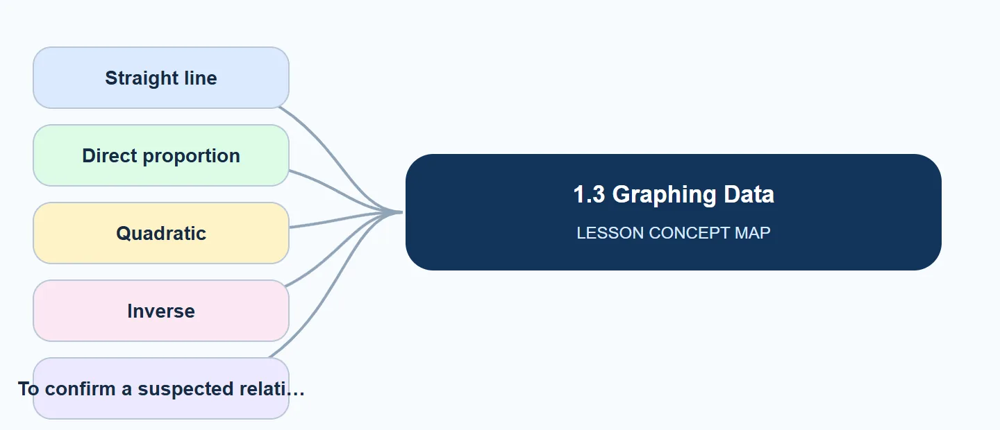
1.3 Graphing Data concept map: Straight line, Direct proportion, Quadratic, Inverse, To confirm a suspected relati
Visual guide to the key ideas explained in this lesson.
Graphs show patterns in data far more clearly than tables and allow values to be predicted.
The independent variable is changed by the experimenter; the dependent variable is measured; all other variables are controlled.
Axis labels take the form quantity / unit (e.g. mass / kg). Scales must be linear and should not use awkward steps like 3 or 7 per square.
If all points lie near a straight line, the relationship is linear. If the line passes through the origin, the variables are directly proportional.
The slope of a straight line is the same everywhere; it tells how much y changes per unit of x. Its units come from the axes (e.g. m/s for distance vs time).
A curve that gets steeper (parabola) suggests a quadratic relationship; a curve that falls steeply and then levels off without touching the axes suggests an inverse relationship.
To confirm a suspected relationship, linearise it
To confirm a suspected relationship, linearise it plot y against x2 for a quadratic, or y against 1/x for an inverse. A straight line through the origin confirms it.
Interpolation (inside the data range) is reliable; extrapolation (beyond it) assumes the pattern continues and may be wrong.
Anomalous points should be circled, checked, and ignored when drawing the best-fit line.
Graphs are mathematical models
Graphs are mathematical models the equation of the best-fit line summarises the experiment and can be used to make predictions.

Part 4 of 7Process & sequence

1
Identify the independent variable (x-axis) and dependent variable (y-axis).
2
Label each axis with the quantity and unit, e.g. "time / s".
3
Choose a linear scale so that the data fill at least half of the grid in each direction (use steps of 1, 2 or 5 per square).
4
Plot each point accurately with a small cross or dot.
5
Draw a single thin line of best fit (straight or smooth curve); do not join dot-to-dot, and ignore anomalies.
6
For a straight line, find the slope using a large triangle: slope = rise/run, with units.
7
Read the y-intercept and write the equation of the line y = mx + b; interpret slope and intercept physically.

Finding the slope of a straight-line graphwrite these steps in this order; each step is a marking point.

1
Draw the line of best fit through the plotted points.
2
Choose two points on the line (not data points) far apart.
3
Draw a large right-angled triangle between them.
4
Read the rise (Δy) and the run (Δx) with units.
5
Divide rise by run and state the slope with units (y-unit/x-unit).

Part 5 of 7Worked examples

Worked examples
L = (2.0 cm/N)F + 8.0 cm
A spring's length L (cm) against load F (N) gives a straight line through (0 N, 8.0 cm) and (5.0 N, 18.0 cm). Find the equation of the line.
  • Slope m = (18.0 − 8.0)/(5.0 − 0) = 10.0/5.0 = 2.0 cm/N.
    • Intercept b = 8.0 cm (the unstretched length).
    • Equation: L = (2.0 cm/N)F + 8.0 cm.
Using that equation, predict the length for a load of 3.5 N.
  • L = 2.0 × 3.5 + 8.0 = 7.0 + 8.0 = 15 cm (interpolation, so reliable).
For an inverse relationship y
For an inverse relationship y a/x, y = 12 when x = 2.0. Find y when x = 6.0.
  • a = xy = 2.0 × 12 = 24. y = 24/6.0 = 4.0. (Tripling x divides y by 3.)

Part 6 of 7Summary

1
Plot the independent variable on x, dependent on y; label axes with units.
2
A straight line has equation y = mx + b; slope = rise/run.
3
Direct proportion is a straight line through the origin.
4
Quadratic graphs are parabolas; inverse graphs are hyperbolas.
5
Draw a line of best fit, never dot-to-dot.

Part 7 of 7Compare: Compare

Common relationships
RelationshipEquationShape of graphPhysics example
Lineary = mx + bStraight line, intercept bLength of spring vs load
Direct proportiony = kxStraight line through originDistance vs time at constant speed
Quadraticy = ax2 + bx + cParabolaDistance fallen vs time from rest
Inversey = a/xHyperbola, approaches both axesTime to travel fixed distance vs speed

To test y = a/x, plot y against 1/x: a straight line through the origin confirms it. To test y ∝ x2, plot y against x2.

Key terms

Command terms

Command terms
Identify / Describe (FRQ)
A short, specific statement; describing requires relevant characteristics, not a single word.
Explain / Justify (FRQ)
Give the cause-and-effect reasoning or evidence; a restated fact does not score.
Calculate
Show setup, substitution and the answer with units.
Predict
State the expected outcome; add a reason only if asked to justify.
MCQ technique
Read every option; eliminate distractors that are true statements but do not answer the question; watch for NOT/EXCEPT.

Exam technique

Keywords the mark scheme looks for in this lesson

Keywords the mark scheme looks for in this lesson
Independent variable · Dependent variable · Control variable · Line of best fit · Linear relationship · Directly proportional · Slope (gradient) · y-intercept · Quadratic relationship · Inverse relationship · Interpolation · Extrapolation · Anomalous result
Learn each definition in the Key words tab exactly; a missing keyword in a definition usually loses the mark.

How to get full marks (examiner guidance)

1
Answer exactly what is asked; extra correct material does not earn credit, and contradictory statements can cancel credit (AP FRQ).
2
Use precise vocabulary, never “it/stuff/things”.
3
Show units and working in calculations.
4
In MCQs, predict the answer before reading the options, then eliminate.

Words to avoid

1
join the pointsdraw a smooth line of best fit.
2
y increases with x so it is proportionalit is directly proportional only if the straight line passes through the origin.
3
slope = run/riseslope = rise/run = Δy/Δx.
4
axis label "time""time / s".
5
a curve going down is inverseit is inverse only if x × y is constant (check by plotting y against 1/x).

Last updated: