Curriculum
Mathematics
Unit 1
0/12
1.1Key terms1.2Laws and key relationships1.3Rigorous Derivation of Reciprocal Trigonometric Functions1.4Logarithmic and General Exponential Differentiation Techniques1.5Parametric and Implicit Second-Order Derivatives1.6Worked examples1.7Exam tips1.8Real-world applications1.9Key Scientific Tables & Anatomical Diagrams Extracted from Official Curricula1.10📌 Comprehensive Scientific Terminology Dictionary:1.11🔍 In-Depth Explanations, Deductions & Multi-Book Insights:1.12Lesson summary
Unit 2
0/141.1The counting principle1.2Permutations (nPr)1.3Combinations (nCr)1.4Worked examples on counting, permutations and combinations1.5Recall: counting principle, permutations and combinations1.61-1 (a) Pascal's triangle and the binomial expansion1.71-1 (b) The general term1.81-1 (c) The middle term1.91-2 The term containing xk and the term free of x1.101-3 (a) The ratio between two consecutive terms1.111-3 (b) The greatest term1.12Key Scientific Tables & Anatomical Diagrams Extracted from Official Curricula1.13Lesson 1 - Counting Principle, Permutations and Combinations and the Binomial Theorem1.14Lesson summary
Unit 3
0/131.1Key terms1.2Laws and key relationships1.3Geometry of 3D Vectors and Scalar/Cross Product Physics1.4Equations of Straight Lines in Three Dimensions1.5Equations of Planes and Perpendicular Distance Formulas1.6Worked examples1.7Exam tips1.8Real-world applications1.9Key Scientific Tables & Anatomical Diagrams Extracted from Official Curricula1.10📌 Comprehensive Scientific Terminology Dictionary:1.11⚖️ Governing Physical Laws & Mathematical Relations:1.12🔍 In-Depth Explanations, Deductions & Multi-Book Insights:1.13Lesson summary
Unit 4
0/81.11 Smooth and rough surfaces1.22 Properties of the static friction force1.33 Kinetic friction force1.44 The resultant reaction R′1.55 The angle of friction1.66 Equilibrium of a body on a rough horizontal plane1.77 Equilibrium of a body on a rough inclined plane1.88 Conditions of equilibrium and rigid bodies with friction
Unit 5
0/121.13-1 (a) Indefinite integrals of exponential functions1.23-1 (b) Indefinite integrals of logarithmic functions1.33-2 (a) The differential and the standard integrals1.43-2 (b) Integration by substitution1.53-2 (c) Integration by parts1.63-2 (d) Applications of the indefinite integral1.73-3 (a) The definite integral and the fundamental theorem of calculus1.83-3 (b) Properties of the definite integral1.93-3 (c) Definite integral by substitution, odd and even functions1.103-4 (a) Area of a plane region1.113-4 (b) Volumes of solids of revolution1.12Key Scientific Tables & Anatomical Diagrams Extracted from Official Curricula
Unit 6
0/81.12-1 (a) Polar coordinates and the Argand plane1.22-1 (b) Modulus, amplitude and principal amplitude1.32-1 (c) The trigonometric (polar) form of a complex number1.42-1 (d) Product and quotient in trigonometric form1.52-1 (e) The exponential (Euler) form1.62-2 (a) De Moivre's theorem for a positive integer power1.72-2 (b) De Moivre's theorem for a rational power and the roots of a complex number1.82-3 The cube roots of unity
Unit 7
0/101.11 Momentum and its change1.22 Newton's first law, inertia and force1.33 Newton's second law, the equation of motion and variable mass1.44 Newton's third law, lifts and scales1.55 Bodies connected by a string over a smooth pulley1.66 Impulse1.77 Work1.88 Kinetic energy and the work-energy principle1.99 Potential energy and conservation of energy1.1010 Power
Text lesson
Statistics, Conditional Probability and Random Variables
Statistics, Conditional Probability and Random Variables
Basic probability and events
Basic probability and events
- An experiment is an action with a set of possible results.
- The set of all possible results is the sample space, written S.
- An event is any subset of S.
- If all results are equally likely, the probability of an event E is the number of favourable outcomes divided by the total number of outcomes:
P(E) = n(E) ÷ n(S)
- Every probability lies between 0 and 1. The probability of the complement of an event A
- written A′
- is:
P(A′) = 1 − P(A)
- For two events A and B
- the addition rule is:
P(A ∪ B) = P(A) + P(B) − P(A ∩ B)
- The term P(A ∩ B) is subtracted because outcomes in both events were counted twice.
- If A and B cannot happen together (mutually exclusive events), then P(A ∩ B) = 0 and the rule becomes P(A ∪ B) = P(A) + P(B).
Reading a statistics table
- Data about a class or a survey is often given in a two-way table.
- Before finding a probability, decide which total is the sample space.
- For example, if 40 students are asked about sports, the total 40 is the denominator for any probability about a random student, but a smaller total is needed when the question starts with a condition.
Statistics, Conditional Probability and Random Variables · 1 / 7
Conditional probability and independence
Conditional probability and independence
- Conditional probability is the probability of an event A when we already know that another event B has happened.
- It is written P(A | B), read as “the probability of A given B”.
- The formula is:
P(A | B) = P(A ∩ B) ÷ P(B), where P(B) > 0
- The idea is that once B has happened, the sample space shrinks from S to B. Only the part of A that lies inside B still matters.
- The multiplication rule follows from the same formula:
P(A ∩ B) = P(B) × P(A | B)
- Two events A and B are independent when knowing that one has happened does not change the probability of the other.
- This is tested by:
P(A ∩ B) = P(A) × P(B), or equivalently,
- P(A | B) = P(A), when P(B) > 0.
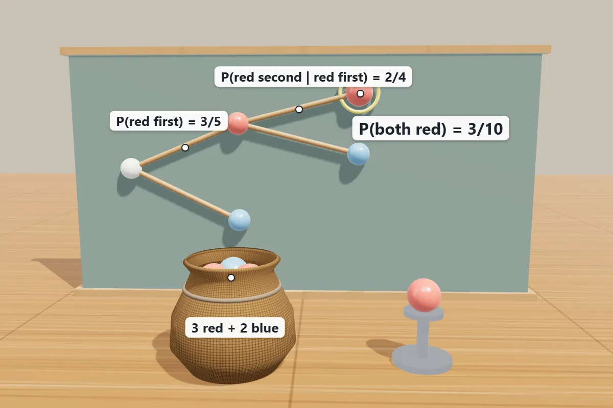
- Tree diagrams help when the events happen in stages.
- Multiply along each branch, then add the branches that give the event you want.
- When the first draw is not replaced, the probabilities of the second stage depend on the first result, so they must be updated.
Statistics, Conditional Probability and Random Variables · 2 / 7
Discrete random variables
Discrete random variables
- A random variable is a rule that gives a number to each outcome of a random experiment.
- It is discrete when its possible values can be listed, such as 0, 1, 2, 3.
- A probability distribution lists each value x with its probability P(X = x).
- Two checks are always needed:
- Each probability satisfies 0 ≤ P(X = x) ≤ 1.
- The probabilities add to 1, so the sum of all P(X = x) equals 1.
Expected value (mean)
- The expected value of X
- written E(X) or μ
- is a weighted average of the values:
E(X) = Σ x × P(X = x)
- E(X) is the long-run average of X over many repetitions.
- It is not always a value that X can actually take.
- For example, the expected number of heads in two coin tosses is 1, although 1 is one of the possible values.
Variance and standard deviation
- The variance measures how far the values spread around the mean. It can be found in two equal ways:
- Var(X) = Σ (x − μ)2 × P(X = x) = E(X2) − μ2
- Here E(X2) = Σ x2 × P(X = x). The standard deviation is σ = √Var(X)
- and it has the same unit as X.
Statistics, Conditional Probability and Random Variables · 3 / 7
Binomial and normal-type distributions
Binomial and normal-type distributions
The binomial distribution
- A binomial experiment has a fixed number of trials n, each trial has only two outcomes (success or failure), the trials are independent, and the probability of success p is the same in every trial.
- If X is the number of successes, then for k = 0, 1, …, n:
P(X = k) = C(n, k) × pᵏ × (1 − p)n−ᵏ
- The mean of a binomial distribution is μ = np
- and its variance is np(1 − p).
Normal-type (bell-shaped) distributions
- Many measured quantities, such as heights or test scores, form a symmetric bell-shaped curve.
- Such a distribution is described by its mean μ and standard deviation σ.
- For a normal distribution, about 68% of the values lie within one standard deviation of the mean, about 95% within two, and about 99.7% within three.
- The z-score of a value x is:
z = (x − μ) ÷ σ
- A z-score tells how many standard deviations x is above or below the mean.
- Positive z means above the mean, and negative z means below it.
Statistics, Conditional Probability and Random Variables · 4 / 7
Worked examples
Worked examples
| Comparison aspect | Main idea | Keywords |
|---|---|---|
| Example 1 (basic probability). | A bag has 4 red and 6 blue balls. One ball is picked at random. Find P(red) | blueballsballpicked |
| Solution |
| Checkblue |
| Example 2 (complement and addition). |
| groupFind |
| Solution | P(A ∪ B) = 0.6 + 0.5 − 0.2 = 0.9. Also P(A′) = 1 − 0.6 = 0.4 | |
| Example 3 (conditional probability). |
| Amongstudentsplayfootball |
| Solution |
| conditionfootballplayersform |
| Comparison aspect | Main idea | Keywords |
|---|---|---|
| Example 4 (independence). |
| independent |
| Solution | P(A) × P(B) = 0.3 × 0.5 = 0.15 = P(A ∩ B). So A and B are independent | independent |
| Example 5 (two draws without replacement). | A box has 3 red and 2 blue balls. Two balls are drawn one after the other without replacement. Find the probability that both are red | blueballsdrawnafter |
| Solution |
| firstdrawgivesAfter |
| Example 6 (expected value and variance). |
| faircoinstossednumber |
| Comparison aspect | Main idea | Keywords |
|---|---|---|
| Solution | E(X) = 0 × 1/4 + 1 × 1/2 + 2 × 1/4 = 1. Then E(X2) = 0 × 1/4 + 1 × 1/2 + 4 × 1/4 = 3/2. So Var(X) = 3/2 − 12 = 1/2 | Then |
| Example 7 (binomial probability). |
| faircointossedtimes |
| Solution |
| meanvariance |
| Example 8 (harder discrete distribution). |
| randomvariabletakesvalues |
| Solution |
| probabilitiesThenNext |
| Comparison aspect | Main idea | Keywords |
|---|---|---|
| Example 9 (normal-type data). |
| heightsstudentsapproximatelymean |
| Solution |
| studentstandarddeviationsabove |
Statistics, Conditional Probability and Random Variables · 5 / 7
Common mistakes
Common mistakes
- Reversing the condition. P(A | B) is not the same as P(B | A). In Example 3 the two values are 2/5 and 5/9.
- Multiplying probabilities for events that are not independent. Without replacement, the second probability changes after the first draw.
- Forgetting that the probabilities of a distribution must add to 1. Always check this before finding E(X).
- Using E(X2) as the variance, or forgetting to subtract μ2. The variance is E(X2) − μ2, not E(X2).
- Using p in the binomial formula where 1 − p is needed for failures. The exponent of (1 − p) is n − k, not k.
Statistics, Conditional Probability and Random Variables · 6 / 7
Lesson summary
Lesson summary
- Probability of an event is favourable outcomes divided by all outcomes, when outcomes are equally likely.
- P(A ∪ B) = P(A) + P(B) − P(A ∩ B), and P(A′) = 1 − P(A).
- Conditional probability P(A | B) = P(A ∩ B) ÷ P(B). Events are independent when P(A ∩ B) = P(A) × P(B).
- For a discrete random variable, E(X) = Σ x P(X = x) and Var(X) = E(X2) − [E(X)]2.
- A binomial distribution with n trials and success probability p has mean np and P(X = k) = C(n, k) pᵏ (1 − p)n−ᵏ.
- A z-score z = (x − μ) ÷ σ measures how far a value is from the mean in standard deviations.
Statistics, Conditional Probability and Random Variables · 7 / 7
Well done! You finished this lesson
What would you like to do next?