IGCSE, Edexcel, IB and AP Science Courses | Dr Dabour Hub Academy

Overview

Explain why measures of central tendency alone are not enough and what a measure of dispersion adds.
Compute the range, the quartiles, the interquartile range and represent them in a box plot.
Compute the variance and the standard deviation for raw data, a simple frequency table and a grouped distribution.
Compare two data sets, predict the effect of adding or multiplying every value, and choose the suitable measure in the presence of outliers.

Measures of Dispersion
├── 4-1 Recap of central tendency (mean, median, mode)
├── 4-2 The need for dispersion
├── 4-3 The range (raw data, frequency table, stem-and-leaf)
├── 4-4 Quartiles and the interquartile range
├── 4-5 The box plot
├── 4-6 Deviation, variance and standard deviation
│   ├── raw values
│   ├── simple frequency distribution
│   └── grouped classes with midpoints
├── 4-7 Using the scientific calculator
├── 4-8 Comparing two data sets
├── 4-9 Effect of adding or multiplying on the measures
└── 4-10 Outliers and choosing a measure

Unit 4: Statistics — Measures of Dispersion · 1 / 14

4-1 Measures of central tendency: recap

Comparison aspect	Main idea	Keywords
Mean	x̄ = (sum of the values) ÷ (their number) for a frequency table x̄ = Σfx ÷ Σf	valuesnumberfrequencytable
Median	the middle value after sorting the data with an even count it is the mean of the two central values	middlevalueaftersorting
Mode	the most frequent value a set may have no mode or more than one	mostfrequentvalue
•	All three describe the centre only — they say nothing about how the values are spread	threedescribecentrenothing

Unit 4: Statistics — Measures of Dispersion · 2 / 14

4-2 Why do we need measures of dispersion?

Two data sets can share the same mean and still behave very differently: {10, 10, 10} and {1, 10, 19} both have mean 10, but the second is far more spread out.
A measure of dispersion quantifies how scattered the values are around the centre, which is what consistency, risk and stability mean in real decisions.
Examples of decisions that need dispersion choosing the more consistent player, the machine with steadier output, or the investment with less variability.

Unit 4: Statistics — Measures of Dispersion · 3 / 14

4-3 The range

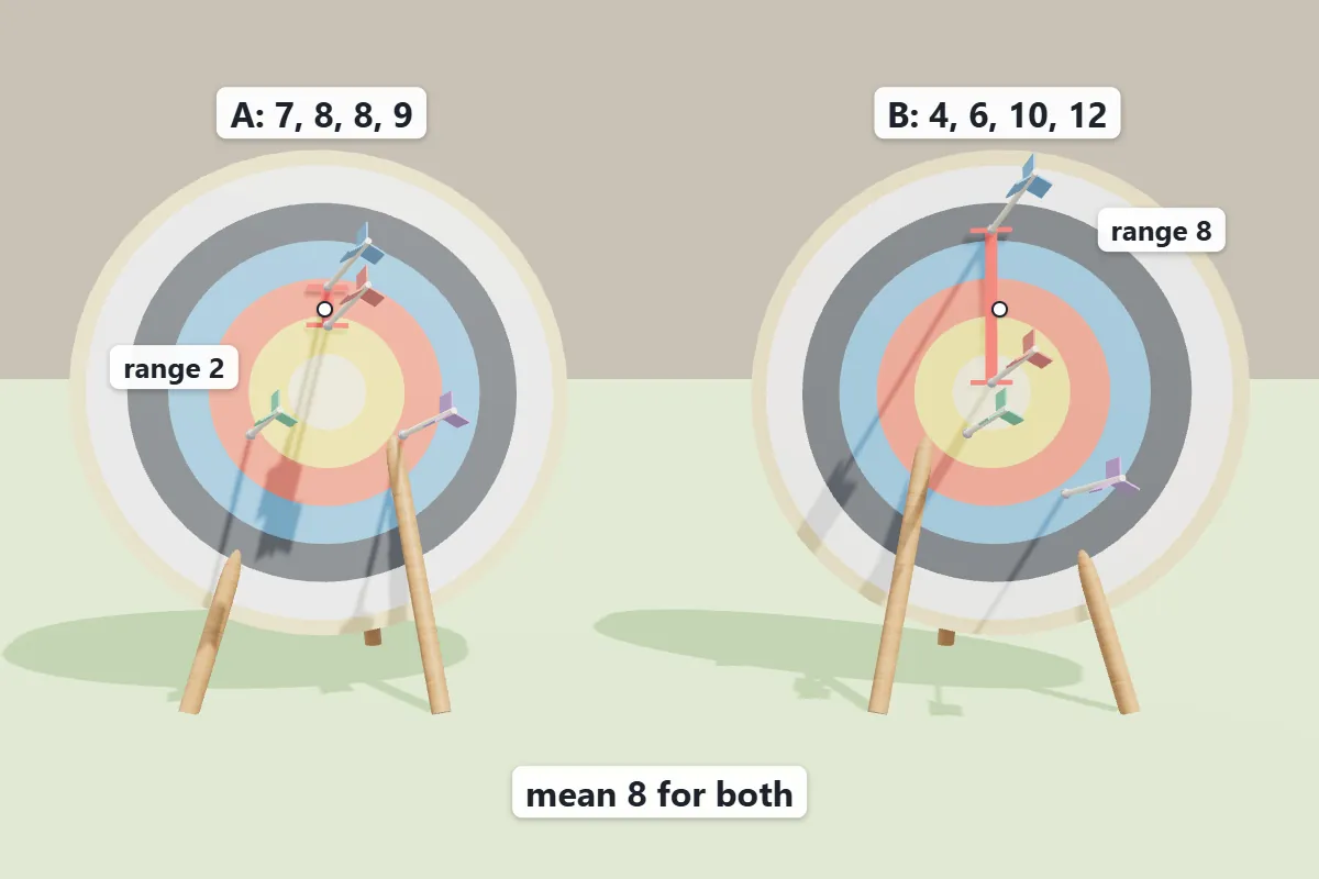
Statistics: two archery targets with close and wide arrows show measures of dispersion and the range: range 2 against 8 with the same mean 8.

Range = greatest value − least value ; it uses only two numbers, so it is easy but sensitive to extreme values.
From a frequency table read the largest and smallest value with a non-zero frequency, not the largest frequency.
From a stem-and-leaf plot the extremes are the first and last leaves with their stems.
For a continuous class interval, the range is usually taken as the difference between the upper boundary of the last class and the lower boundary of the first class.
The range carries the same unit as the data (it is not squared).

Unit 4: Statistics — Measures of Dispersion · 4 / 14

4-4 The median recap, quartiles and the interquartile range

Sort the data, then split it Q1 is the median of the lower half, Q2 is the median of the whole set, Q3 the median of the upper half.
Interquartile range (IQR) = Q3 − Q1 the spread of the middle 50% of the data, and unlike the range it is not distorted by extreme values.
When the count is odd, the common school convention excludes the middle value from both halves.
Half of the data always lies inside the interval [Q1, Q3], which is why the IQR is used to judge consistency of the bulk of the observations.

Data 4, 6, 7, 9, 14 sorted→median Q2 = 7, lower half {4, 6} → Q1 = 5, upper half {9, 14} → Q3 = 11.5, so IQR = 6.5 and range = 10.

Unit 4: Statistics — Measures of Dispersion · 5 / 14

4-5 The box plot (box-and-whisker)

A box plot is drawn from exactly five numbers the minimum, Q1, the median, Q3 and the maximum.
The box spans Q1 to Q3 (so its length is the IQR), the line inside the box is the median, and the whiskers reach the least and greatest values.
Reading it a longer box means more spread in the middle 50%; a whisker much longer than the other signals a possible outlier; the side on which the median line sits shows where the data concentrate.
Two box plots on the same axis compare the two distributions at a glance — position (median) and spread (box length) together.

Unit 4: Statistics — Measures of Dispersion · 6 / 14

4-6 Deviation, variance and standard deviation of a set of values

The deviation of a value is x − x̄; the deviations always sum to zero, which is why they are squared.
Variance σ² = Σ(x − x̄)² / n and standard deviation σ = √σ² — the SD returns to the original unit of the data, so it is the more usable number.
σ = 0 only when all the values are equal; the larger σ, the more scattered the data.
Shortcut formula σ² = (Σx²/n) − (x̄)² — often faster and less rounded.

For 4, 6, 7, 9, 14→x̄ = 8; the squared deviations are 16, 4, 1, 1, 36 with sum 58, so σ² = 58/5 = 11.6 and σ ≈ 3.41.

Unit 4: Statistics — Measures of Dispersion · 7 / 14

4-7 Standard deviation of a simple frequency distribution

Comparison aspect	Main idea	Keywords
Work with columns x, f, fx and fx²	n = Σf x̄ = Σfx/Σf and σ² = Σfx²/Σf − (x̄)²	Σfx²
Each squared deviation is weighted by its frequency	σ² = Σf(x − x̄)² / Σf — the two forms give the same result	formsgivesameresult
•	Build the table fully before substituting a single wrong fx² entry moves the final answer	Buildtablefullybefore

Unit 4: Statistics — Measures of Dispersion · 8 / 14

4-8 Standard deviation of a grouped (class) distribution

Replace each class by its midpoint x = (lower + upper)/2 and treat the table as a frequency distribution with those midpoints.
Then apply σ² = Σfx²/Σf − (Σfx/Σf)²; the answer is an estimate because the real values inside a class are unknown.
Use class boundaries, not the printed limits, when computing midpoints of continuous classes such as 10–19, 20–29.
Quartiles of grouped data are read from the cumulative-frequency curve or located in the class containing the required position.

Unit 4: Statistics — Measures of Dispersion · 9 / 14

4-9 Using the scientific calculator

Enter statistics mode (usually MODE → STAT → 1-VAR), type each value with its frequency, then read x̄, σn (population SD) and σn−1 (sample SD) from the menu.
The syllabus uses σn (divide by n); do not copy σn−1 (divide by n − 1) by mistake.
Frequencies are entered through the frequency column; forgetting it treats each value as appearing once.
Keep the unrounded calculator value until the final step, then round to the required number of decimal places.

Unit 4: Statistics — Measures of Dispersion · 10 / 14

4-10 Comparing two data sets

Compare centre with the mean (or median) and consistency with the standard deviation or the IQR: the smaller the dispersion, the more consistent the performance.
Standard deviation is in the data’s unit, so it is directly comparable only when the two means are close; otherwise use the coefficient of variation CV = (σ / x̄) × 100% and pick the smaller percentage.
Typical wording “which player is more consistent?” — the answer is the one with the smaller SD/IQR, even if his mean score is lower.
Justify with numbers in the answer sentence; a bare name earns no mark.

Unit 4: Statistics — Measures of Dispersion · 11 / 14

4-11 Effect of adding or multiplying every value

Comparison aspect	Main idea	Example	Keywords
Adding a constant c to every value	the mean and median increase by c quartiles increase by c but the range IQR and standard deviation do not change — the spread is only shifted	—	meanmedianincreasequartiles
Multiplying every value by k	mean median quartiles range IQR and SD are all multiplied by \|k\| and the variance is multiplied by k²	—	meanmedianquartilesrange
•	Change of unit (	metres to centimetres) is a multiplication by 100 so SD ×100 and variance ×10 000 while the coefficient of variation stays unchanged	Changeunitmetrescentimetres

Unit 4: Statistics — Measures of Dispersion · 12 / 14

4-12 Outliers and choosing the right measure

An outlier is a value far removed from the rest; it drags the mean and inflates the standard deviation and the range, but barely affects the median and the IQR.
A common test flags a value as an outlier if it lies below Q1 − 1.5 × IQR or above Q3 + 1.5 × IQR.
When an outlier is present (or the distribution is heavily skewed), report the median with the IQR; otherwise the mean with the standard deviation is the better pair.
Never delete an outlier silently either justify its removal (measurement error) or keep it and switch to the robust measures.

Unit 4: Statistics — Measures of Dispersion · 13 / 14

Exam traps and key takeaways

💡 High-yield traps

Equal means do not mean equal data — dispersion is the missing information.
Deviations sum to zero; that is exactly why we square them.
Variance is in squared units; the standard deviation restores the original unit.
Range uses extremes only, so one outlier changes it completely; the IQR does not.
For an even number of values the median is the mean of the two middle values — not their sum, and not the value between them in position only.
In a frequency table the range uses the smallest and largest values with non-zero frequency.
σ² = Σfx²/Σf − (x̄)² subtract the square of the mean, not the square of Σfx.
For grouped data use midpoints and call the result an estimate.
Calculator choose σn, not σn−1.
Adding a constant leaves SD unchanged; multiplying scales SD by |k| and variance by k².
More consistent = smaller SD / smaller IQR, not the larger mean.
Compare different-scaled data with the coefficient of variation, not with raw SD.

Unit 4: Statistics — Measures of Dispersion · 14 / 14

Curriculum

Mathematics — Third Preparatory

Unit 1

Unit 2

Unit 3

Unit 4

Unit 4: Statistics — Measures of Dispersion