Curriculum
AP Physics C: Electricity AND Magnetism
8. Electric Charges, Fields, and Gauss’s Law
0/13
9. Electric Potential
0/7
-
9. Electric Potential
 Preview
-
9.1 Electric Potential Energy
Preview
-
9.1 Electric Potential Energy - Check yourself
 Preview
-
9.2 Electric Potential
Preview
-
9.2 Electric Potential - Check yourself
Preview
-
9.3 Conservation of Electric Energy
Preview
-
9.3 Conservation of Electric Energy - Check yourself
Preview
10. Conductors and Capacitors
0/9
11. Electric Circuits
0/17
12. Magnetic Fields and Electromagnetism
0/9
13. Electromagnetic Induction
0/13
Text lesson
9.2 Electric Potential
9.2 Electric Potential — AP PHYSICS C: ELECTRICITY AND MAGNETISM notes: You will be able to describe electric potential as the electric potential energy per unit charge at a point, calculate the potential of point charges and of continuous charge distributions by superposition and integration, and relate potential difference to the electric field through ΔV = −∫E · dr.
1
It describes the field region itself, so it does not depend on any particular charge placed there.
2
If a test charge q at a point has electric potential energy U, the electric potential at that point is V = U/q.
3
Electric potential is measured in volts (V), where 1 V = 1 J/C.
4
The potential of a single point charge Q at distance r from it is V = kQ/r, with k = 9.0 × 10⁹ N·m2/C2, Q in coulombs, and r in metres.
5
The potential is positive near a positive charge and negative near a negative charge, and it falls off as 1/r.
6
The reference is zero at infinity, as in Topic 9.1.
7
Electric potential is a scalar.
8
It has a sign but no direction, so it can be added directly, with the signs of the charges kept.
9
The electric field is a vector and is a different quantity, which is explained below.
Each term is found separately, with its own sign and distance, and the terms are then added as numbers.
Superposition of potential is simpler than superposition of field.
To find the field, each contribution must be resolved into components before it is added.
To find the potential, no components are needed.
This makes potential the more convenient quantity to calculate first, after which the field can be found by differentiation.
1
For a continuous distribution the sum becomes an integral over small elements of charge.
2
Each element dq at distance r contributes dV = k dq/r, and the total potential is V = ∫ k dq/r, taken over the whole distribution.
3
The method is to write dq in terms of a single variable, express r in the same variable, and integrate.
4
A thin ring of total charge Q and radius R gives a useful result on its axis.
5
Every element of the ring is at the same distance √(z2 + R2) from a point on the axis at distance z from the centre, so the integral is simple: V = kQ/√(z2 + R2).
6
At the centre of the ring, z = 0 and V = kQ/R.
7
A semicircular arc of radius R and total charge Q has a uniform linear charge density λ = Q/(πR).
8
At its centre, dq = λR dθ and every element is at distance R, so dV = kλ dθ and V = kλπ = kQ/R.
9
The same result holds for any arc of radius R and total charge Q, because the angle cancels when λ is written in terms of Q.
10
A finite uniform line of charge Q and length L has λ = Q/L.
11
At a point on the line’s extended axis, a distance a beyond its nearest end, the distance to an element at position x is x measured from the point, and the potential is V = ∫aa + L kλ dx/x = kλ ln[(a + L)/a].
12
At a point a distance d from the midpoint of the line, on its perpendicular bisector, the result is V = 2kλ ln{[L/2 + √((L/2)2 + d2)]/d}.
13
An infinitely long, uniformly charged wire or cylinder has a field of magnitude E = 2kλ/r at distance r from its central axis, where λ is the charge per unit length.
14
Integrating the field gives V(r) = V(r0) − 2kλ ln(r/r0).
15
The potential is defined only up to a constant, so a reference distance r0 must be chosen.
16
The infinite distribution cannot use infinity as its zero point.
1
It is the same for every test charge, because the test charge cancels.
2
The potential difference is measured in volts, and it depends only on the field between the two points.
3
The potential difference between points A and B is ΔV = −∫AB E · dr.
4
Two points separated by a region of field have a potential difference that is set by the field along the path between them.
5
Because the field is conservative, the result depends only on the two endpoints.
6
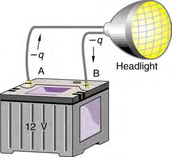
Potential difference can also be produced by chemical processes.
7
In a battery, chemical reactions separate positive and negative charges and do work on them, establishing a potential difference between the terminals.
8
A 1.5 V cell transfers 1.5 J of energy to each coulomb of charge that it moves through the external circuit.
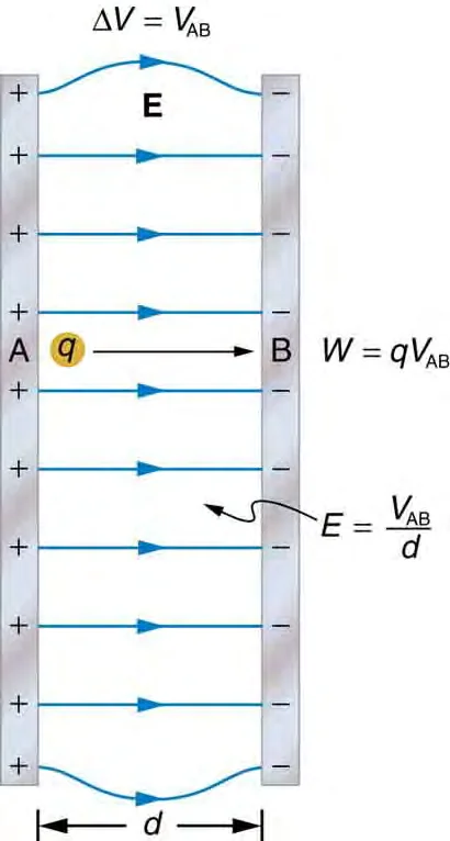
In three dimensions the field is the negative gradient of the potential, but for one-dimensional problems the derivative is enough.
The minus sign means that the field points in the direction in which the potential decreases.
This relation can be used in both directions.
Given a potential function, the field is found by differentiation.
Given a field, the potential difference is found by integration.
For example, a field of 400 N/C along x between x = 0 and x = 0.050 m gives ΔV = −400 × 0.050 = −20 V.
Equipotential lines (isolines of potential) join points that have the same potential.
No work is done by the field when a charge moves along an equipotential line, because there is no change in potential energy.
Therefore the field has no component along an isoline, and every field line crosses the equipotential lines at right angles.
An isoline map can be drawn from a field-vector map, and a field-line map can be drawn from an isoline map.
Field vectors always point toward lower potential.
These maps can therefore be used to predict motion a positive charge released from rest accelerates along the field, toward lower potential, and a negative charge accelerates against the field, toward higher potential.
1
V = k(q1/r1 + q2/r2) = (9.0 × 10⁹)(4.0 × 10⁻⁹/0.30 − 6.0 × 10⁻⁹/0.50) = (9.0 × 10⁹)(1.333 × 10⁻⁸ − 1.20 × 10⁻⁸) = (9.0 × 10⁹)(1.33 × 10⁻⁹) = 12 V.
Answer
V = 12 V. The contribution of +4.0 nC is +120 V and that of −6.0 nC is −108 V the sum is 12 V
1
Every element of the ring is at distance √(0.302 + 0.102) = √0.10 m from the point, so V = ∫ k dq/√0.10 = kQ/√0.10 = (9.0 × 10⁹)(2.0 × 10⁻⁶)/0.3162 = 5.7 × 10⁴ V
2
Differentiating with respect to z, V = kQ(z2 + R2)−1/2, so Ez = −dV/dz = kQz/(z2 + R2)3/2 = (9.0 × 10⁹)(2.0 × 10⁻⁶)(0.30)/(0.10)3/2 = 1.7 × 10⁵ N/C.
Answer
V = 5.7 × 10⁴ V and E = 1.7 × 10⁵ N/C, directed away from the ring.
1
λ = Q/L = 6.0 × 10⁻⁹/0.30 = 2.0 × 10⁻⁸ C/m, so kλ = 180 V
2
Integrating from the near end, V = ∫0.300.60 kλ dx/x = kλ ln(0.60/0.30) = 180 × ln 2 = 180 × 0.693 = 125 V.
Answer
V = 1.2 × 10² V.
1
Ex = −dV/dx = −(10x − 3.0) = 3.0 − 10x (V/m)
2
At x = 0.20 m, Ex = 3.0 − 2.0 = 1.0 V/m
3
The field is zero when 3.0 − 10x = 0, so x = 0.30 m.
Answer
Ex = +1.0 V/m at 0.20 m, so the field points in the +x direction, toward lower potential. The field is zero at x = 0.30 m.
Adding potentials as vectors
Potential is a scalar, so the contributions from several charges are added as signed numbers, with no components.
Assuming that zero potential means zero field
At the midpoint between equal and opposite charges the potential is zero, but the field is not zero, because both charges push the field in the same direction.
Forgetting the sign of the charge in V = kq/r
A negative charge gives a negative potential.
Using the point-charge formula for an extended distribution without integrating
The formula applies to each element dq, and the elements must then be summed.
Dropping the minus sign in Ex = −dV/dx
The field points toward decreasing potential, so reversing the sign gives the wrong direction.
Assuming that equipotential lines and field lines are parallel
They are perpendicular, because a field component along an isoline would change the potential.