Curriculum
AP Physics C: Mechanics
1. Kinematics
0/11
-
1. Kinematics
 Preview
-
1.1 Scalars and Vectors in One Dimension
Preview
-
1.1 Scalars and Vectors in One Dimension - Check yourself
 Preview
-
1.2 Displacement, Velocity, and Acceleration
Preview
-
1.2 Displacement, Velocity, and Acceleration - Check yourself
Preview
-
1.3 Representing Motion
Preview
-
1.3 Representing Motion - Check yourself
Preview
-
1.4 Reference Frames and Relative Motion
Preview
-
1.4 Reference Frames and Relative Motion - Check yourself
Preview
-
1.5 Motion in Two or Three Dimensions
Preview
-
1.5 Motion in Two or Three Dimensions - Check yourself
Preview
2. Force and Translational Dynamics
0/21
3. Work, Energy, and Power
0/11
4. Linear Momentum
0/9
5. Torque and Rotational Dynamics
0/13
6. Energy and Momentum of Rotating Systems
0/13
7. Oscillations
0/11
Text lesson
1.3 Representing Motion
1.3 Representing Motion — AP PHYSICS C: MECHANICS notes: You will be able to describe the position, velocity and acceleration of an object using motion diagrams, graphs and equations, relate the slopes and areas of position, velocity and acceleration graphs, and apply the constant-acceleration equations to motion in one dimension.
1Motion diagrams and narrative descriptions2Motion diagrams and narrative descriptions
1Slopes and areas on position, velocity and acceleration grap2Slopes and areas on position, velocity and acceleration grap3Slopes and areas on position, velocity and acceleration grap4Slopes and areas on position, velocity and acceleration grap5Slopes and areas on position, velocity and acceleration grap
Slopes and areas on position, velocity and acceleration graphs
Slopes and areas on position, velocity and acceleration graphs
The instantaneous velocity of an object is the rate of change of its position
which is equal to the slope of the tangent line at a point on a graph of position against time: vx = dx/dt.
1 / 5Next ▶
Slopes and areas on position, velocity and acceleration graphs
Slopes and areas on position, velocity and acceleration graphs
A horizontal tangent means zero velocity, and a steeper tangent means a larger speed.
The sign of the slope gives the direction of motion.
The instantaneous acceleration is the rate of change of velocity
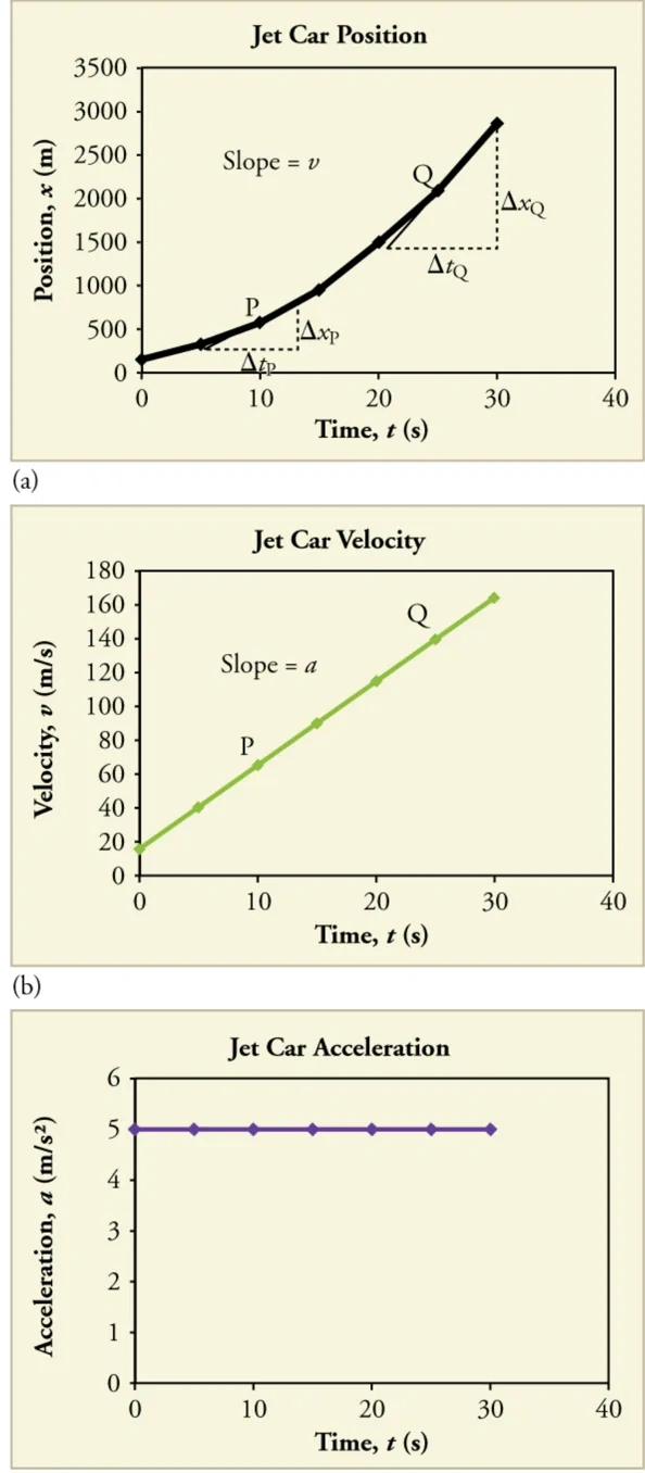
which is equal to the slope of the tangent line at a point on a graph of velocity against time: ax = dvx/dt. A velocity–time graph that is a straight line has constant acceleration, and the acceleration equals its slope.
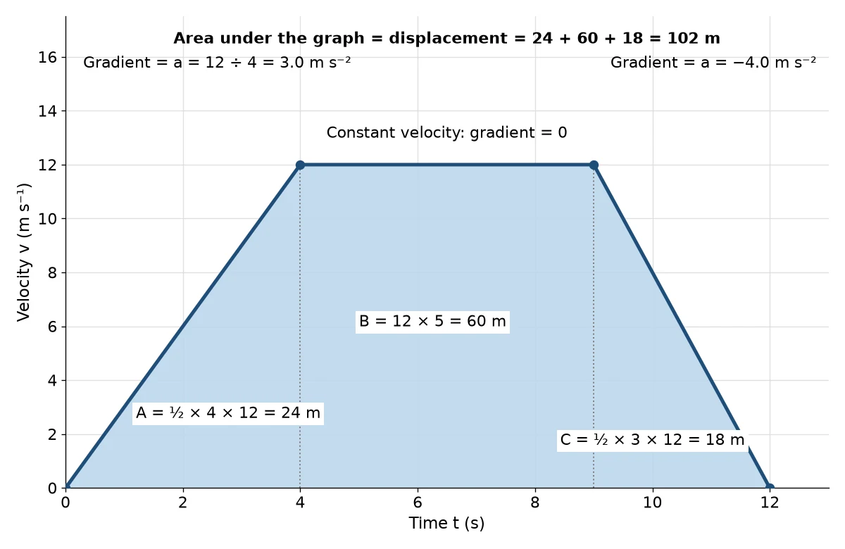
The displacement of an object over a time interval is the area under its velocity–time graph between the initial and final times: Δx = ∫t1t2 vx(t) dt.
Area above the time axis is counted as positive displacement and area below the axis as negative displacement.
Similarly, the change in velocity over an interval is the area under the acceleration–time graph: Δ
◀ Previous2 / 5Next ▶
Slopes and areas on position, velocity and acceleration graphs
1
v
2
x
3
= ∫
4
t1
5
t2
6
a
◀ Previous3 / 5Next ▶
Slopes and areas on position, velocity and acceleration graphs
1
(
2
t
3
) d
4
.
5
A position–time graph that is a parabola corresponds to a velocity–time graph that is a straight line,
6
and this is the usual pattern for constant acceleration.
◀ Previous4 / 5Next ▶
Velocity-time graph of a trapezoid: uniform acceleration, constant velocity, then deceleration, with the shaded area giving 102 m.
Slopes and areas on position, velocity and acceleration graphs
◀ Previous5 / 5
1The constant-acceleration equations2The constant-acceleration equations3The constant-acceleration equations4The constant-acceleration equations5The constant-acceleration equations6The constant-acceleration equations7The constant-acceleration equations
The constant-acceleration equations
1
When the acceleration is constant, the velocity and position functions can be found by integration.
2
1
3
Since d
4
v
5
x
6
/d
1 / 7Next ▶
The constant-acceleration equations
The constant-acceleration equations
t
=
a
, integrating gives
x0
+
◀ Previous2 / 7Next ▶
The constant-acceleration equations
The constant-acceleration equations
.
2
, integrating again gives
0
+ ½
3
◀ Previous3 / 7Next ▶
The constant-acceleration equations
1
Eliminating
2
between the velocity equation and the position equation gives
3
+ 2
4
(
5
−
6
).
◀ Previous4 / 7Next ▶
The constant-acceleration equations
1
4
2
Here
3
and
4
are the position and velocity at
5
= 0, positions are in metres, velocities in metres per second and accelerations in metres per second squared.
6
These three equations describe instantaneous linear motion in one dimension with constant acceleration, and they can be used along any single axis as appropriate.
◀ Previous5 / 7Next ▶
The constant-acceleration equations
The constant-acceleration equations
Each equation contains only some of the six quantities
,
so a problem can be solved by choosing the equation that omits the unknown quantity.
The equations do not apply when the acceleration changes with time
in that case the integrals must be evaluated.
◀ Previous6 / 7Next ▶
Graphs of motion when acceleration is constant but velocity changes: Three linked graphs for a car with constant acceleration: position against time curves upward, velocity against time is a rising straight line, and acceleration against time is a flat horizontal line.
The constant-acceleration equations
◀ Previous7 / 7
1Free fall and gravity near the surface of Earth2Free fall and gravity near the surface of Earth3Free fall and gravity near the surface of Earth
1Motion in several stages2Motion in several stages
Motion in several stages
1
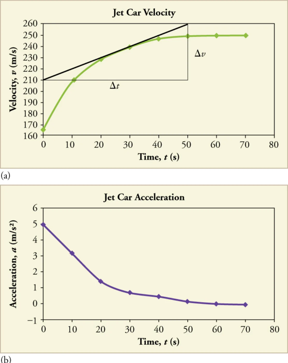
When the acceleration changes, the motion is divided into intervals in which the acceleration is constant.
2
1
3
The final velocity and position at the end of one interval become the initial velocity and position of the next.
4
2
5
Each stage must be analysed separately, and the total displacement is the sum of the displacements in the stages.
6
3
1 / 2Next ▶
Graphs of motion where acceleration is not constant: Velocity against time for the jet car levelling off at its top speed, and the matching acceleration against time falling to zero.
Motion in several stages
 ⤢ Enlarge
Motion in several stages
A velocity–time graph of the whole motion is often the clearest way to check that the stages join correctly.
◀ Previous2 / 2
1Example 1: Displacement and distance from a velocity–time gr2Example 1: Displacement and distance from a velocity–time gr3Example 1: Displacement and distance from a velocity–time gr4Example 2: Constant acceleration from rest5Worked examples6Worked examples7Worked examples8Example 3: Vertical motion under gravity9Example 3: Vertical motion under gravity10Example 3: Vertical motion under gravity11Example 4: Motion in three stages12Example 4: Motion in three stages
Key terms
| Term | Meaning |
|---|---|
| Motion diagram | A representation of an object’s motion as dots showing its position at equal time intervals. |
| Tangent line | A straight line that touches a curve at one point, whose slope gives the instantaneous rate of change at that point. |
| Slope of a position–time graph | The instantaneous velocity, equal to dx/dt. |
| Area under a velocity–time graph | The displacement over the interval, counting area below the time axis as negative. |
| Constant-acceleration equations | The three kinematic equations that relate vx, x, ax and t when the acceleration is constant. |
| Free fall | Motion under the force of gravity alone, with downward acceleration of magnitude g near Earth’s surface. |
| Acceleration due to gravity (g) | The constant downward acceleration near Earth’s surface, taken as 10 m/s2 for AP numerical problems. |
| Sign convention | A chosen direction for positive values, which must be used consistently for all quantities in a problem. |
| Piecewise motion | Motion divided into stages with different constant accelerations, joined by the final state of one stage. |
1Avoid these mistakes2Avoid these mistakes3Avoid these mistakes4Avoid these mistakes