Curriculum
College Physics for AP Courses 2e
Unit 1: Introduction: The Nature of Science and Physics
0/10
-
Unit 1 overview: Introduction: The Nature of Science and Physics
 Text lessonPreview
-
1.1 Physics: An Introduction
Text lessonPreview
-
1.1 Physics: An Introduction - Check yourself
 6 questionsPreview
-
1.2 Physical Quantities and Units
Text lessonPreview
-
1.2 Physical Quantities and Units - Check yourself
6 questionsPreview
-
1.3 Accuracy, Precision, and Significant Figures
Text lessonPreview
-
1.3 Accuracy, Precision, and Significant Figures - Check yourself
6 questionsPreview
-
1.4 Approximation
Text lessonPreview
-
1.4 Approximation - Check yourself
6 questionsPreview
-
Unit 1 review quiz: Introduction: The Nature of Science and Physics
10 questionsPreview
Unit 2: Kinematics
0/18
-
Unit 2 overview: Kinematics
Text lessonPreview
-
2.1 Displacement
Text lessonPreview
-
2.1 Displacement - Check yourself
6 questionsPreview
-
2.2 Vectors, Scalars, and Coordinate Systems
Text lessonPreview
-
2.2 Vectors, Scalars, and Coordinate Systems - Check yourself
6 questionsPreview
-
2.3 Time, Velocity, and Speed
Text lessonPreview
-
2.3 Time, Velocity, and Speed - Check yourself
6 questionsPreview
-
2.4 Acceleration
Text lessonPreview
-
2.4 Acceleration - Check yourself
6 questionsPreview
-
2.5 Motion Equations for Constant Acceleration in One Dimension
Text lessonPreview
-
2.5 Motion Equations for Constant Acceleration in One Dimension - Check yourself
6 questionsPreview
-
2.6 Problem-Solving Basics for One-Dimensional Kinematics
Text lessonPreview
-
2.6 Problem-Solving Basics for One-Dimensional Kinematics - Check yourself
6 questionsPreview
-
2.7 Falling Objects
Text lessonPreview
-
2.7 Falling Objects - Check yourself
6 questionsPreview
-
2.8 Graphical Analysis of One-Dimensional Motion
Text lessonPreview
-
2.8 Graphical Analysis of One-Dimensional Motion - Check yourself
6 questionsPreview
-
Unit 2 review quiz: Kinematics
10 questionsPreview
Unit 3: Two-Dimensional Kinematics
0/12
-
Unit 3 overview: Two-Dimensional Kinematics
Text lessonPreview
-
3.1 Kinematics in Two Dimensions: An Introduction
Text lessonPreview
-
3.1 Kinematics in Two Dimensions: An Introduction - Check yourself
6 questionsPreview
-
3.2 Vector Addition and Subtraction: Graphical Methods
Text lessonPreview
-
3.2 Vector Addition and Subtraction: Graphical Methods - Check yourself
6 questionsPreview
-
3.3 Vector Addition and Subtraction: Analytical Methods
Text lessonPreview
-
3.3 Vector Addition and Subtraction: Analytical Methods - Check yourself
6 questionsPreview
-
3.4 Projectile Motion
Text lessonPreview
-
3.4 Projectile Motion - Check yourself
6 questionsPreview
-
3.5 Addition of Velocities
Text lessonPreview
-
3.5 Addition of Velocities - Check yourself
6 questionsPreview
-
Unit 3 review quiz: Two-Dimensional Kinematics
10 questionsPreview
Unit 4: Dynamics: Force and Newton's Laws of Motion
0/18
-
Unit 4 overview: Dynamics: Force and Newton's Laws of Motion
Text lessonPreview
-
4.1 Development of Force Concept
Text lessonPreview
-
4.1 Development of Force Concept - Check yourself
6 questionsPreview
-
4.2 Newton’s First Law of Motion: Inertia
Text lessonPreview
-
4.2 Newton’s First Law of Motion: Inertia - Check yourself
6 questionsPreview
-
4.3 Newton’s Second Law of Motion: Concept of a System
Text lessonPreview
-
4.3 Newton’s Second Law of Motion: Concept of a System - Check yourself
6 questionsPreview
-
4.4 Newton’s Third Law of Motion: Symmetry in Forces
Text lessonPreview
-
4.4 Newton’s Third Law of Motion: Symmetry in Forces - Check yourself
6 questionsPreview
-
4.5 Normal, Tension, and Other Examples of Forces
Text lessonPreview
-
4.5 Normal, Tension, and Other Examples of Forces - Check yourself
6 questionsPreview
-
4.6 Problem-Solving Strategies
Text lessonPreview
-
4.6 Problem-Solving Strategies - Check yourself
6 questionsPreview
-
4.7 Further Applications of Newton’s Laws of Motion
Text lessonPreview
-
4.7 Further Applications of Newton’s Laws of Motion - Check yourself
6 questionsPreview
-
4.8 Extended Topic: The Four Basic Forces—An Introduction
Text lessonPreview
-
4.8 Extended Topic: The Four Basic Forces—An Introduction - Check yourself
6 questionsPreview
-
Unit 4 review quiz: Dynamics: Force and Newton's Laws of Motion
10 questionsPreview
Unit 5: Further Applications of Newton's Laws: Friction, Drag, and Elasticity
0/8
-
Unit 5 overview: Further Applications of Newton's Laws: Friction, Drag, and Elasticity
Text lessonPreview
-
5.1 Friction
Text lessonPreview
-
5.1 Friction - Check yourself
6 questionsPreview
-
5.2 Drag Forces
Text lessonPreview
-
5.2 Drag Forces - Check yourself
6 questionsPreview
-
5.3 Elasticity: Stress and Strain
Text lessonPreview
-
5.3 Elasticity: Stress and Strain - Check yourself
6 questionsPreview
-
Unit 5 review quiz: Further Applications of Newton's Laws: Friction, Drag, and Elasticity
10 questionsPreview
Unit 6: Uniform Circular Motion and Gravitation
0/14
-
Unit 6 overview: Uniform Circular Motion and Gravitation
Text lessonPreview
-
6.1 Rotation Angle and Angular Velocity
Text lessonPreview
-
6.1 Rotation Angle and Angular Velocity - Check yourself
6 questionsPreview
-
6.2 Centripetal Acceleration
Text lessonPreview
-
6.2 Centripetal Acceleration - Check yourself
6 questionsPreview
-
6.3 Centripetal Force
Text lessonPreview
-
6.3 Centripetal Force - Check yourself
6 questionsPreview
-
6.4 Fictitious Forces and Non-inertial Frames: The Coriolis Force
Text lessonPreview
-
6.4 Fictitious Forces and Non-inertial Frames: The Coriolis Force - Check yourself
6 questionsPreview
-
6.5 Newton’s Universal Law of Gravitation
Text lessonPreview
-
6.5 Newton’s Universal Law of Gravitation - Check yourself
6 questionsPreview
-
6.6 Satellites and Kepler’s Laws: An Argument for Simplicity
Text lessonPreview
-
6.6 Satellites and Kepler’s Laws: An Argument for Simplicity - Check yourself
6 questionsPreview
-
Unit 6 review quiz: Uniform Circular Motion and Gravitation
10 questionsPreview
Unit 7: Work, Energy, and Energy Resources
0/20
-
Unit 7 overview: Work, Energy, and Energy Resources
Text lessonPreview
-
7.1 Work: The Scientific Definition
Text lessonPreview
-
7.1 Work: The Scientific Definition - Check yourself
6 questionsPreview
-
7.2 Kinetic Energy and the Work-Energy Theorem
Text lessonPreview
-
7.2 Kinetic Energy and the Work-Energy Theorem - Check yourself
6 questionsPreview
-
7.3 Gravitational Potential Energy
Text lessonPreview
-
7.3 Gravitational Potential Energy - Check yourself
6 questionsPreview
-
7.4 Conservative Forces and Potential Energy
Text lessonPreview
-
7.4 Conservative Forces and Potential Energy - Check yourself
6 questionsPreview
-
7.5 Nonconservative Forces
Text lessonPreview
-
7.5 Nonconservative Forces - Check yourself
6 questionsPreview
-
7.6 Conservation of Energy
Text lessonPreview
-
7.6 Conservation of Energy - Check yourself
6 questionsPreview
-
7.7 Power
Text lessonPreview
-
7.7 Power - Check yourself
6 questionsPreview
-
7.8 Work, Energy, and Power in Humans
Text lessonPreview
-
7.8 Work, Energy, and Power in Humans - Check yourself
6 questionsPreview
-
7.9 World Energy Use
Text lessonPreview
-
7.9 World Energy Use - Check yourself
6 questionsPreview
-
Unit 7 review quiz: Work, Energy, and Energy Resources
10 questionsPreview
Unit 8: Linear Momentum and Collisions
0/32
-
Unit 8 overview: Linear Momentum and Collisions
Text lessonPreview
-
8.1 Linear Momentum and Force
Text lessonPreview
-
8.1 Linear Momentum and Force - Check yourself
6 questionsPreview
-
8.1 Linear Momentum and Force
Text lessonPreview
-
8.1 Linear Momentum and Force - Check yourself
6 questionsPreview
-
8.2 Impulse
Text lessonPreview
-
8.2 Impulse - Check yourself
6 questionsPreview
-
8.2 Impulse
Text lessonPreview
-
8.2 Impulse - Check yourself
6 questionsPreview
-
8.3 Conservation of Momentum
Text lessonPreview
-
8.3 Conservation of Momentum - Check yourself
6 questionsPreview
-
8.3 Conservation of Momentum
Text lessonPreview
-
8.3 Conservation of Momentum - Check yourself
6 questionsPreview
-
8.4 Elastic Collisions in One Dimension
Text lessonPreview
-
8.4 Elastic Collisions in One Dimension - Check yourself
6 questionsPreview
-
Unit 8 review quiz: Linear Momentum and Collisions
10 questionsPreview
-
Unit 8 overview: Linear Momentum and Collisions
Text lessonPreview
-
8.4 Elastic Collisions in One Dimension
Text lessonPreview
-
8.4 Elastic Collisions in One Dimension - Check yourself
6 questionsPreview
-
8.5 Inelastic Collisions in One Dimension
Text lessonPreview
-
8.5 Inelastic Collisions in One Dimension - Check yourself
6 questionsPreview
-
8.5 Inelastic Collisions in One Dimension
Text lessonPreview
-
8.5 Inelastic Collisions in One Dimension - Check yourself
6 questionsPreview
-
8.6 Collisions of Point Masses in Two Dimensions
Text lessonPreview
-
8.6 Collisions of Point Masses in Two Dimensions - Check yourself
6 questionsPreview
-
8.6 Collisions of Point Masses in Two Dimensions
Text lessonPreview
-
8.6 Collisions of Point Masses in Two Dimensions - Check yourself
6 questionsPreview
-
8.7 Introduction to Rocket Propulsion
Text lessonPreview
-
8.7 Introduction to Rocket Propulsion - Check yourself
6 questionsPreview
-
8.7 Introduction to Rocket Propulsion
Text lessonPreview
-
8.7 Introduction to Rocket Propulsion - Check yourself
6 questionsPreview
-
Unit 8 review quiz: Linear Momentum and Collisions
10 questionsPreview
Unit 9: Statics and Torque
0/28
-
Unit 9 overview: Statics and Torque
Text lessonPreview
-
9.1 The First Condition for Equilibrium
Text lessonPreview
-
9.1 The First Condition for Equilibrium - Check yourself
6 questionsPreview
-
9.1 The First Condition for Equilibrium
Text lessonPreview
-
9.1 The First Condition for Equilibrium - Check yourself
6 questionsPreview
-
9.2 The Second Condition for Equilibrium
Text lessonPreview
-
9.2 The Second Condition for Equilibrium - Check yourself
6 questionsPreview
-
9.2 The Second Condition for Equilibrium
Text lessonPreview
-
9.2 The Second Condition for Equilibrium - Check yourself
6 questionsPreview
-
9.3 Stability
Text lessonPreview
-
9.3 Stability - Check yourself
6 questionsPreview
-
9.3 Stability
Text lessonPreview
-
9.3 Stability - Check yourself
6 questionsPreview
-
Unit 9 review quiz: Statics and Torque
10 questionsPreview
-
Unit 9 overview: Statics and Torque
Text lessonPreview
-
9.4 Applications of Statics, Including Problem-Solving Strategies
Text lessonPreview
-
9.4 Applications of Statics, Including Problem-Solving Strategies - Check yourself
6 questionsPreview
-
9.4 Applications of Statics, Including Problem-Solving Strategies
Text lessonPreview
-
9.4 Applications of Statics, Including Problem-Solving Strategies - Check yourself
6 questionsPreview
-
9.5 Simple Machines
Text lessonPreview
-
9.5 Simple Machines - Check yourself
6 questionsPreview
-
9.5 Simple Machines
Text lessonPreview
-
9.5 Simple Machines - Check yourself
6 questionsPreview
-
9.6 Forces and Torques in Muscles and Joints
Text lessonPreview
-
9.6 Forces and Torques in Muscles and Joints - Check yourself
6 questionsPreview
-
9.6 Forces and Torques in Muscles and Joints
Text lessonPreview
-
9.6 Forces and Torques in Muscles and Joints - Check yourself
6 questionsPreview
-
Unit 9 review quiz: Statics and Torque
10 questionsPreview
Unit 10: Rotational Motion and Angular Momentum
0/32
-
Unit 10 overview: Rotational Motion and Angular Momentum
Text lessonPreview
-
10.1 Angular Acceleration
Text lessonPreview
-
10.1 Angular Acceleration - Check yourself
6 questionsPreview
-
10.1 Angular Acceleration
Text lessonPreview
-
10.1 Angular Acceleration - Check yourself
6 questionsPreview
-
10.2 Kinematics of Rotational Motion
Text lessonPreview
-
10.2 Kinematics of Rotational Motion - Check yourself
6 questionsPreview
-
10.2 Kinematics of Rotational Motion
Text lessonPreview
-
10.2 Kinematics of Rotational Motion - Check yourself
6 questionsPreview
-
10.3 Dynamics of Rotational Motion: Rotational Inertia
Text lessonPreview
-
10.3 Dynamics of Rotational Motion: Rotational Inertia - Check yourself
6 questionsPreview
-
10.3 Dynamics of Rotational Motion: Rotational Inertia
Text lessonPreview
-
10.3 Dynamics of Rotational Motion: Rotational Inertia - Check yourself
6 questionsPreview
-
10.4 Rotational Kinetic Energy: Work and Energy Revisited
Text lessonPreview
-
10.4 Rotational Kinetic Energy: Work and Energy Revisited - Check yourself
6 questionsPreview
-
Unit 10 review quiz: Rotational Motion and Angular Momentum
10 questionsPreview
-
Unit 10 overview: Rotational Motion and Angular Momentum
Text lessonPreview
-
10.4 Rotational Kinetic Energy: Work and Energy Revisited
Text lessonPreview
-
10.4 Rotational Kinetic Energy: Work and Energy Revisited - Check yourself
6 questionsPreview
-
10.5 Angular Momentum and Its Conservation
Text lessonPreview
-
10.5 Angular Momentum and Its Conservation - Check yourself
6 questionsPreview
-
10.5 Angular Momentum and Its Conservation
Text lessonPreview
-
10.5 Angular Momentum and Its Conservation - Check yourself
6 questionsPreview
-
10.6 Collisions of Extended Bodies in Two Dimensions
Text lessonPreview
-
10.6 Collisions of Extended Bodies in Two Dimensions - Check yourself
6 questionsPreview
-
10.6 Collisions of Extended Bodies in Two Dimensions
Text lessonPreview
-
10.6 Collisions of Extended Bodies in Two Dimensions - Check yourself
6 questionsPreview
-
10.7 Gyroscopic Effects: Vector Aspects of Angular Momentum
Text lessonPreview
-
10.7 Gyroscopic Effects: Vector Aspects of Angular Momentum - Check yourself
6 questionsPreview
-
10.7 Gyroscopic Effects: Vector Aspects of Angular Momentum
Text lessonPreview
-
10.7 Gyroscopic Effects: Vector Aspects of Angular Momentum - Check yourself
6 questionsPreview
-
Unit 10 review quiz: Rotational Motion and Angular Momentum
10 questionsPreview
Unit 11: Fluid Statics
0/40
-
Unit 11 overview: Fluid Statics
Text lessonPreview
-
11.1 What Is a Fluid?
Text lessonPreview
-
11.1 What Is a Fluid? - Check yourself
6 questionsPreview
-
11.1 What Is a Fluid?
Text lessonPreview
-
11.1 What Is a Fluid? - Check yourself
6 questionsPreview
-
11.2 Density
Text lessonPreview
-
11.2 Density - Check yourself
6 questionsPreview
-
11.2 Density
Text lessonPreview
-
11.2 Density - Check yourself
6 questionsPreview
-
11.3 Pressure
Text lessonPreview
-
11.3 Pressure - Check yourself
6 questionsPreview
-
11.3 Pressure
Text lessonPreview
-
11.3 Pressure - Check yourself
6 questionsPreview
-
11.4 Variation of Pressure with Depth in a Fluid
Text lessonPreview
-
11.4 Variation of Pressure with Depth in a Fluid - Check yourself
6 questionsPreview
-
11.4 Variation of Pressure with Depth in a Fluid
Text lessonPreview
-
11.4 Variation of Pressure with Depth in a Fluid - Check yourself
6 questionsPreview
-
11.5 Pascal’s Principle
Text lessonPreview
-
11.5 Pascal’s Principle - Check yourself
6 questionsPreview
-
Unit 11 review quiz: Fluid Statics
10 questionsPreview
-
Unit 11 overview: Fluid Statics
Text lessonPreview
-
11.5 Pascal’s Principle
Text lessonPreview
-
11.5 Pascal’s Principle - Check yourself
6 questionsPreview
-
11.6 Gauge Pressure, Absolute Pressure, and Pressure Measurement
Text lessonPreview
-
11.6 Gauge Pressure, Absolute Pressure, and Pressure Measurement - Check yourself
6 questionsPreview
-
11.6 Gauge Pressure, Absolute Pressure, and Pressure Measurement
Text lessonPreview
-
11.6 Gauge Pressure, Absolute Pressure, and Pressure Measurement - Check yourself
6 questionsPreview
-
11.7 Archimedes’ Principle
Text lessonPreview
-
11.7 Archimedes’ Principle - Check yourself
6 questionsPreview
-
11.7 Archimedes’ Principle
Text lessonPreview
-
11.7 Archimedes’ Principle - Check yourself
6 questionsPreview
-
11.8 Cohesion and Adhesion in Liquids: Surface Tension and Capillary Action
Text lessonPreview
-
11.8 Cohesion and Adhesion in Liquids: Surface Tension and Capillary Action - Check yourself
6 questionsPreview
-
11.8 Cohesion and Adhesion in Liquids: Surface Tension and Capillary Action
Text lessonPreview
-
11.8 Cohesion and Adhesion in Liquids: Surface Tension and Capillary Action - Check yourself
6 questionsPreview
-
11.9 Pressures in the Body
Text lessonPreview
-
11.9 Pressures in the Body - Check yourself
6 questionsPreview
-
11.9 Pressures in the Body
Text lessonPreview
-
11.9 Pressures in the Body - Check yourself
6 questionsPreview
-
Unit 11 review quiz: Fluid Statics
10 questionsPreview
Unit 12: Fluid Dynamics and Its Biological and Medical Applications
0/32
-
Unit 12 overview: Fluid Dynamics and Its Biological and Medical Applications
Text lessonPreview
-
12.1 Flow Rate and Its Relation to Velocity
Text lessonPreview
-
12.1 Flow Rate and Its Relation to Velocity - Check yourself
6 questionsPreview
-
12.1 Flow Rate and Its Relation to Velocity
Text lessonPreview
-
12.1 Flow Rate and Its Relation to Velocity - Check yourself
6 questionsPreview
-
12.2 Bernoulli’s Equation
Text lessonPreview
-
12.2 Bernoulli’s Equation - Check yourself
6 questionsPreview
-
12.2 Bernoulli’s Equation
Text lessonPreview
-
12.2 Bernoulli’s Equation - Check yourself
6 questionsPreview
-
12.3 The Most General Applications of Bernoulli’s Equation
Text lessonPreview
-
12.3 The Most General Applications of Bernoulli’s Equation - Check yourself
6 questionsPreview
-
12.3 The Most General Applications of Bernoulli’s Equation
Text lessonPreview
-
12.3 The Most General Applications of Bernoulli’s Equation - Check yourself
6 questionsPreview
-
12.4 Viscosity and Laminar Flow; Poiseuille’s Law
Text lessonPreview
-
12.4 Viscosity and Laminar Flow; Poiseuille’s Law - Check yourself
6 questionsPreview
-
Unit 12 review quiz: Fluid Dynamics and Its Biological and Medical Applications
10 questionsPreview
-
Unit 12 overview: Fluid Dynamics and Its Biological and Medical Applications
Text lessonPreview
-
12.4 Viscosity and Laminar Flow; Poiseuille’s Law
Text lessonPreview
-
12.4 Viscosity and Laminar Flow; Poiseuille’s Law - Check yourself
6 questionsPreview
-
12.5 The Onset of Turbulence
Text lessonPreview
-
12.5 The Onset of Turbulence - Check yourself
6 questionsPreview
-
12.5 The Onset of Turbulence
Text lessonPreview
-
12.5 The Onset of Turbulence - Check yourself
6 questionsPreview
-
12.6 Motion of an Object in a Viscous Fluid
Text lessonPreview
-
12.6 Motion of an Object in a Viscous Fluid - Check yourself
6 questionsPreview
-
12.6 Motion of an Object in a Viscous Fluid
Text lessonPreview
-
12.6 Motion of an Object in a Viscous Fluid - Check yourself
6 questionsPreview
-
12.7 Molecular Transport Phenomena: Diffusion, Osmosis, and Related Processes
Text lessonPreview
-
12.7 Molecular Transport Phenomena: Diffusion, Osmosis, and Related Processes - Check yourself
6 questionsPreview
-
12.7 Molecular Transport Phenomena: Diffusion, Osmosis, and Related Processes
Text lessonPreview
-
12.7 Molecular Transport Phenomena: Diffusion, Osmosis, and Related Processes - Check yourself
6 questionsPreview
-
Unit 12 review quiz: Fluid Dynamics and Its Biological and Medical Applications
10 questionsPreview
Unit 13: Temperature, Kinetic Theory, and the Gas Laws
0/28
-
Unit 13 overview: Temperature, Kinetic Theory, and the Gas Laws
Text lessonPreview
-
13.1 Temperature
Text lessonPreview
-
13.1 Temperature - Check yourself
6 questionsPreview
-
13.1 Temperature
Text lessonPreview
-
13.1 Temperature - Check yourself
6 questionsPreview
-
13.2 Thermal Expansion of Solids and Liquids
Text lessonPreview
-
13.2 Thermal Expansion of Solids and Liquids - Check yourself
6 questionsPreview
-
13.2 Thermal Expansion of Solids and Liquids
Text lessonPreview
-
13.2 Thermal Expansion of Solids and Liquids - Check yourself
6 questionsPreview
-
13.3 The Ideal Gas Law
Text lessonPreview
-
13.3 The Ideal Gas Law - Check yourself
6 questionsPreview
-
13.3 The Ideal Gas Law
Text lessonPreview
-
13.3 The Ideal Gas Law - Check yourself
6 questionsPreview
-
Unit 13 review quiz: Temperature, Kinetic Theory, and the Gas Laws
10 questionsPreview
-
Unit 13 overview: Temperature, Kinetic Theory, and the Gas Laws
Text lessonPreview
-
13.4 Kinetic Theory: Atomic and Molecular Explanation of Pressure and Temperature
Text lessonPreview
-
13.4 Kinetic Theory: Atomic and Molecular Explanation of Pressure and Temperature - Check yourself
6 questionsPreview
-
13.4 Kinetic Theory: Atomic and Molecular Explanation of Pressure and Temperature
Text lessonPreview
-
13.4 Kinetic Theory: Atomic and Molecular Explanation of Pressure and Temperature - Check yourself
6 questionsPreview
-
13.5 Phase Changes
Text lessonPreview
-
13.5 Phase Changes - Check yourself
6 questionsPreview
-
13.5 Phase Changes
Text lessonPreview
-
13.5 Phase Changes - Check yourself
6 questionsPreview
-
13.6 Humidity, Evaporation, and Boiling
Text lessonPreview
-
13.6 Humidity, Evaporation, and Boiling - Check yourself
6 questionsPreview
-
13.6 Humidity, Evaporation, and Boiling
Text lessonPreview
-
13.6 Humidity, Evaporation, and Boiling - Check yourself
6 questionsPreview
-
Unit 13 review quiz: Temperature, Kinetic Theory, and the Gas Laws
10 questionsPreview
Unit 14: Heat and Heat Transfer Methods
0/32
-
Unit 14 overview: Heat and Heat Transfer Methods
Text lessonPreview
-
14.1 Heat
Text lessonPreview
-
14.1 Heat - Check yourself
6 questionsPreview
-
14.1 Heat
Text lessonPreview
-
14.1 Heat - Check yourself
6 questionsPreview
-
14.2 Temperature Change and Heat Capacity
Text lessonPreview
-
14.2 Temperature Change and Heat Capacity - Check yourself
6 questionsPreview
-
14.2 Temperature Change and Heat Capacity
Text lessonPreview
-
14.2 Temperature Change and Heat Capacity - Check yourself
6 questionsPreview
-
14.3 Phase Change and Latent Heat
Text lessonPreview
-
14.3 Phase Change and Latent Heat - Check yourself
6 questionsPreview
-
14.3 Phase Change and Latent Heat
Text lessonPreview
-
14.3 Phase Change and Latent Heat - Check yourself
6 questionsPreview
-
14.4 Heat Transfer Methods
Text lessonPreview
-
14.4 Heat Transfer Methods - Check yourself
6 questionsPreview
-
Unit 14 review quiz: Heat and Heat Transfer Methods
10 questionsPreview
-
Unit 14 overview: Heat and Heat Transfer Methods
Text lessonPreview
-
14.4 Heat Transfer Methods
Text lessonPreview
-
14.4 Heat Transfer Methods - Check yourself
6 questionsPreview
-
14.5 Conduction
Text lessonPreview
-
14.5 Conduction - Check yourself
6 questionsPreview
-
14.5 Conduction
Text lessonPreview
-
14.5 Conduction - Check yourself
6 questionsPreview
-
14.6 Convection
Text lessonPreview
-
14.6 Convection - Check yourself
6 questionsPreview
-
14.6 Convection
Text lessonPreview
-
14.6 Convection - Check yourself
6 questionsPreview
-
14.7 Radiation
Text lessonPreview
-
14.7 Radiation - Check yourself
6 questionsPreview
-
14.7 Radiation
Text lessonPreview
-
14.7 Radiation - Check yourself
6 questionsPreview
-
Unit 14 review quiz: Heat and Heat Transfer Methods
10 questionsPreview
Unit 15: Thermodynamics
0/32
-
Unit 15 overview: Thermodynamics
Text lessonPreview
-
15.1 The First Law of Thermodynamics
Text lessonPreview
-
15.1 The First Law of Thermodynamics - Check yourself
6 questionsPreview
-
15.1 The First Law of Thermodynamics
Text lessonPreview
-
15.1 The First Law of Thermodynamics - Check yourself
6 questionsPreview
-
15.2 The First Law of Thermodynamics and Some Simple Processes
Text lessonPreview
-
15.2 The First Law of Thermodynamics and Some Simple Processes - Check yourself
6 questionsPreview
-
15.2 The First Law of Thermodynamics and Some Simple Processes
Text lessonPreview
-
15.2 The First Law of Thermodynamics and Some Simple Processes - Check yourself
6 questionsPreview
-
15.3 Introduction to the Second Law of Thermodynamics: Heat Engines and Their Efficiency
Text lessonPreview
-
15.3 Introduction to the Second Law of Thermodynamics: Heat Engines and Their Efficiency - Check yourself
6 questionsPreview
-
15.3 Introduction to the Second Law of Thermodynamics: Heat Engines and Their Efficiency
Text lessonPreview
-
15.3 Introduction to the Second Law of Thermodynamics: Heat Engines and Their Efficiency - Check yourself
6 questionsPreview
-
15.4 Carnot’s Perfect Heat Engine: The Second Law of Thermodynamics Restated
Text lessonPreview
-
15.4 Carnot’s Perfect Heat Engine: The Second Law of Thermodynamics Restated - Check yourself
6 questionsPreview
-
Unit 15 review quiz: Thermodynamics
10 questionsPreview
-
Unit 15 overview: Thermodynamics
Text lessonPreview
-
15.4 Carnot’s Perfect Heat Engine: The Second Law of Thermodynamics Restated
Text lessonPreview
-
15.4 Carnot’s Perfect Heat Engine: The Second Law of Thermodynamics Restated - Check yourself
6 questionsPreview
-
15.5 Applications of Thermodynamics: Heat Pumps and Refrigerators
Text lessonPreview
-
15.5 Applications of Thermodynamics: Heat Pumps and Refrigerators - Check yourself
6 questionsPreview
-
15.5 Applications of Thermodynamics: Heat Pumps and Refrigerators
Text lessonPreview
-
15.5 Applications of Thermodynamics: Heat Pumps and Refrigerators - Check yourself
6 questionsPreview
-
15.6 Entropy and the Second Law of Thermodynamics: Disorder and the Unavailability of Energy
Text lessonPreview
-
15.6 Entropy and the Second Law of Thermodynamics: Disorder and the Unavailability of Energy - Check yourself
6 questionsPreview
-
15.6 Entropy and the Second Law of Thermodynamics: Disorder and the Unavailability of Energy
Text lessonPreview
-
15.6 Entropy and the Second Law of Thermodynamics: Disorder and the Unavailability of Energy - Check yourself
6 questionsPreview
-
15.7 Statistical Interpretation of Entropy and the Second Law of Thermodynamics: The Underlying Explanation
Text lessonPreview
-
15.7 Statistical Interpretation of Entropy and the Second Law of Thermodynamics: The Underlying Explanation - Check yourself
6 questionsPreview
-
15.7 Statistical Interpretation of Entropy and the Second Law of Thermodynamics: The Underlying Explanation
Text lessonPreview
-
15.7 Statistical Interpretation of Entropy and the Second Law of Thermodynamics: The Underlying Explanation - Check yourself
6 questionsPreview
-
Unit 15 review quiz: Thermodynamics
10 questionsPreview
Unit 16: Oscillatory Motion and Waves
0/48
-
Unit 16 overview: Oscillatory Motion and Waves
Text lessonPreview
-
16.1 Hooke’s Law: Stress and Strain Revisited
Text lessonPreview
-
16.1 Hooke’s Law: Stress and Strain Revisited - Check yourself
6 questionsPreview
-
16.1 Hooke’s Law: Stress and Strain Revisited
Text lessonPreview
-
16.1 Hooke’s Law: Stress and Strain Revisited - Check yourself
6 questionsPreview
-
16.2 Period and Frequency in Oscillations
Text lessonPreview
-
16.2 Period and Frequency in Oscillations - Check yourself
6 questionsPreview
-
16.2 Period and Frequency in Oscillations
Text lessonPreview
-
16.2 Period and Frequency in Oscillations - Check yourself
6 questionsPreview
-
16.3 Simple Harmonic Motion: A Special Periodic Motion
Text lessonPreview
-
16.3 Simple Harmonic Motion: A Special Periodic Motion - Check yourself
6 questionsPreview
-
16.3 Simple Harmonic Motion: A Special Periodic Motion
Text lessonPreview
-
16.3 Simple Harmonic Motion: A Special Periodic Motion - Check yourself
6 questionsPreview
-
16.4 The Simple Pendulum
Text lessonPreview
-
16.4 The Simple Pendulum - Check yourself
6 questionsPreview
-
16.4 The Simple Pendulum
Text lessonPreview
-
16.4 The Simple Pendulum - Check yourself
6 questionsPreview
-
16.5 Energy and the Simple Harmonic Oscillator
Text lessonPreview
-
16.5 Energy and the Simple Harmonic Oscillator - Check yourself
6 questionsPreview
-
16.5 Energy and the Simple Harmonic Oscillator
Text lessonPreview
-
16.5 Energy and the Simple Harmonic Oscillator - Check yourself
6 questionsPreview
-
16.6 Uniform Circular Motion and Simple Harmonic Motion
Text lessonPreview
-
16.6 Uniform Circular Motion and Simple Harmonic Motion - Check yourself
6 questionsPreview
-
Unit 16 review quiz: Oscillatory Motion and Waves
10 questionsPreview
-
Unit 16 overview: Oscillatory Motion and Waves
Text lessonPreview
-
16.6 Uniform Circular Motion and Simple Harmonic Motion
Text lessonPreview
-
16.6 Uniform Circular Motion and Simple Harmonic Motion - Check yourself
6 questionsPreview
-
16.7 Damped Harmonic Motion
Text lessonPreview
-
16.7 Damped Harmonic Motion - Check yourself
6 questionsPreview
-
16.7 Damped Harmonic Motion
Text lessonPreview
-
16.7 Damped Harmonic Motion - Check yourself
6 questionsPreview
-
16.8 Forced Oscillations and Resonance
Text lessonPreview
-
16.8 Forced Oscillations and Resonance - Check yourself
6 questionsPreview
-
16.8 Forced Oscillations and Resonance
Text lessonPreview
-
16.8 Forced Oscillations and Resonance - Check yourself
6 questionsPreview
-
16.9 Waves
Text lessonPreview
-
16.9 Waves - Check yourself
6 questionsPreview
-
16.9 Waves
Text lessonPreview
-
16.9 Waves - Check yourself
6 questionsPreview
-
16.10 Superposition and Interference
Text lessonPreview
-
16.10 Superposition and Interference - Check yourself
6 questionsPreview
-
16.10 Superposition and Interference
Text lessonPreview
-
16.10 Superposition and Interference - Check yourself
6 questionsPreview
-
16.11 Energy in Waves: Intensity
Text lessonPreview
-
16.11 Energy in Waves: Intensity - Check yourself
6 questionsPreview
-
16.11 Energy in Waves: Intensity
Text lessonPreview
-
16.11 Energy in Waves: Intensity - Check yourself
6 questionsPreview
-
Unit 16 review quiz: Oscillatory Motion and Waves
10 questionsPreview
Unit 17: Physics of Hearing
0/32
-
Unit 17 overview: Physics of Hearing
Text lessonPreview
-
17.1 Sound
Text lessonPreview
-
17.1 Sound - Check yourself
6 questionsPreview
-
17.1 Sound
Text lessonPreview
-
17.1 Sound - Check yourself
6 questionsPreview
-
17.2 Speed of Sound, Frequency, and Wavelength
Text lessonPreview
-
17.2 Speed of Sound, Frequency, and Wavelength - Check yourself
6 questionsPreview
-
17.2 Speed of Sound, Frequency, and Wavelength
Text lessonPreview
-
17.2 Speed of Sound, Frequency, and Wavelength - Check yourself
6 questionsPreview
-
17.3 Sound Intensity and Sound Level
Text lessonPreview
-
17.3 Sound Intensity and Sound Level - Check yourself
6 questionsPreview
-
17.3 Sound Intensity and Sound Level
Text lessonPreview
-
17.3 Sound Intensity and Sound Level - Check yourself
6 questionsPreview
-
17.4 Doppler Effect and Sonic Booms
Text lessonPreview
-
17.4 Doppler Effect and Sonic Booms - Check yourself
6 questionsPreview
-
Unit 17 review quiz: Physics of Hearing
10 questionsPreview
-
Unit 17 overview: Physics of Hearing
Text lessonPreview
-
17.4 Doppler Effect and Sonic Booms
Text lessonPreview
-
17.4 Doppler Effect and Sonic Booms - Check yourself
6 questionsPreview
-
17.5 Sound Interference and Resonance: Standing Waves in Air Columns
Text lessonPreview
-
17.5 Sound Interference and Resonance: Standing Waves in Air Columns - Check yourself
6 questionsPreview
-
17.5 Sound Interference and Resonance: Standing Waves in Air Columns
Text lessonPreview
-
17.5 Sound Interference and Resonance: Standing Waves in Air Columns - Check yourself
6 questionsPreview
-
17.6 Hearing
Text lessonPreview
-
17.6 Hearing - Check yourself
6 questionsPreview
-
17.6 Hearing
Text lessonPreview
-
17.6 Hearing - Check yourself
6 questionsPreview
-
17.7 Ultrasound
Text lessonPreview
-
17.7 Ultrasound - Check yourself
6 questionsPreview
-
17.7 Ultrasound
Text lessonPreview
-
17.7 Ultrasound - Check yourself
6 questionsPreview
-
Unit 17 review quiz: Physics of Hearing
10 questionsPreview
Unit 18: Electric Charge and Electric Field
0/36
-
Unit 18 overview: Electric Charge and Electric Field
Text lessonPreview
-
18.1 Static Electricity and Charge: Conservation of Charge
Text lessonPreview
-
18.1 Static Electricity and Charge: Conservation of Charge - Check yourself
6 questionsPreview
-
18.1 Static Electricity and Charge: Conservation of Charge
Text lessonPreview
-
18.1 Static Electricity and Charge: Conservation of Charge - Check yourself
6 questionsPreview
-
18.2 Conductors and Insulators
Text lessonPreview
-
18.2 Conductors and Insulators - Check yourself
6 questionsPreview
-
18.2 Conductors and Insulators
Text lessonPreview
-
18.2 Conductors and Insulators - Check yourself
6 questionsPreview
-
18.3 Conductors and Electric Fields in Static Equilibrium
Text lessonPreview
-
18.3 Conductors and Electric Fields in Static Equilibrium - Check yourself
6 questionsPreview
-
18.3 Conductors and Electric Fields in Static Equilibrium
Text lessonPreview
-
18.3 Conductors and Electric Fields in Static Equilibrium - Check yourself
6 questionsPreview
-
18.4 Coulomb’s Law
Text lessonPreview
-
18.4 Coulomb’s Law - Check yourself
6 questionsPreview
-
18.4 Coulomb’s Law
Text lessonPreview
-
18.4 Coulomb’s Law - Check yourself
6 questionsPreview
-
Unit 18 review quiz: Electric Charge and Electric Field
10 questionsPreview
-
Unit 18 overview: Electric Charge and Electric Field
Text lessonPreview
-
18.5 Electric Field: Concept of a Field Revisited
Text lessonPreview
-
18.5 Electric Field: Concept of a Field Revisited - Check yourself
6 questionsPreview
-
18.5 Electric Field: Concept of a Field Revisited
Text lessonPreview
-
18.5 Electric Field: Concept of a Field Revisited - Check yourself
6 questionsPreview
-
18.6 Electric Field Lines: Multiple Charges
Text lessonPreview
-
18.6 Electric Field Lines: Multiple Charges - Check yourself
6 questionsPreview
-
18.6 Electric Field Lines: Multiple Charges
Text lessonPreview
-
18.6 Electric Field Lines: Multiple Charges - Check yourself
6 questionsPreview
-
18.7 Electric Forces in Biology
Text lessonPreview
-
18.7 Electric Forces in Biology - Check yourself
6 questionsPreview
-
18.7 Electric Forces in Biology
Text lessonPreview
-
18.7 Electric Forces in Biology - Check yourself
6 questionsPreview
-
18.8 Applications of Electrostatics
Text lessonPreview
-
18.8 Applications of Electrostatics - Check yourself
6 questionsPreview
-
18.8 Applications of Electrostatics
Text lessonPreview
-
18.8 Applications of Electrostatics - Check yourself
6 questionsPreview
-
Unit 18 review quiz: Electric Charge and Electric Field
10 questionsPreview
Unit 19: Electric Potential and Electric Field
0/32
-
Unit 19 overview: Electric Potential and Electric Field
Text lessonPreview
-
19.1 Electric Potential Energy: Potential Difference
Text lessonPreview
-
19.1 Electric Potential Energy: Potential Difference - Check yourself
6 questionsPreview
-
19.1 Electric Potential Energy: Potential Difference
Text lessonPreview
-
19.1 Electric Potential Energy: Potential Difference - Check yourself
6 questionsPreview
-
19.2 Electric Potential in a Uniform Electric Field
Text lessonPreview
-
19.2 Electric Potential in a Uniform Electric Field - Check yourself
6 questionsPreview
-
19.2 Electric Potential in a Uniform Electric Field
Text lessonPreview
-
19.2 Electric Potential in a Uniform Electric Field - Check yourself
6 questionsPreview
-
19.3 Electrical Potential Due to a Point Charge
Text lessonPreview
-
19.3 Electrical Potential Due to a Point Charge - Check yourself
6 questionsPreview
-
19.3 Electrical Potential Due to a Point Charge
Text lessonPreview
-
19.3 Electrical Potential Due to a Point Charge - Check yourself
6 questionsPreview
-
19.4 Equipotential Lines
Text lessonPreview
-
19.4 Equipotential Lines - Check yourself
6 questionsPreview
-
Unit 19 review quiz: Electric Potential and Electric Field
10 questionsPreview
-
Unit 19 overview: Electric Potential and Electric Field
Text lessonPreview
-
19.4 Equipotential Lines
Text lessonPreview
-
19.4 Equipotential Lines - Check yourself
6 questionsPreview
-
19.5 Capacitors and Dielectrics
Text lessonPreview
-
19.5 Capacitors and Dielectrics - Check yourself
6 questionsPreview
-
19.5 Capacitors and Dielectrics
Text lessonPreview
-
19.5 Capacitors and Dielectrics - Check yourself
6 questionsPreview
-
19.6 Capacitors in Series and Parallel
Text lessonPreview
-
19.6 Capacitors in Series and Parallel - Check yourself
6 questionsPreview
-
19.6 Capacitors in Series and Parallel
Text lessonPreview
-
19.6 Capacitors in Series and Parallel - Check yourself
6 questionsPreview
-
19.7 Energy Stored in Capacitors
Text lessonPreview
-
19.7 Energy Stored in Capacitors - Check yourself
6 questionsPreview
-
19.7 Energy Stored in Capacitors
Text lessonPreview
-
19.7 Energy Stored in Capacitors - Check yourself
6 questionsPreview
-
Unit 19 review quiz: Electric Potential and Electric Field
10 questionsPreview
Unit 20: Electric Current, Resistance, and Ohm's Law
0/32
-
Unit 20 overview: Electric Current, Resistance, and Ohm's Law
Text lessonPreview
-
20.1 Current
Text lessonPreview
-
20.1 Current - Check yourself
6 questionsPreview
-
20.1 Current
Text lessonPreview
-
20.1 Current - Check yourself
6 questionsPreview
-
20.2 Ohm’s Law: Resistance and Simple Circuits
Text lessonPreview
-
20.2 Ohm’s Law: Resistance and Simple Circuits - Check yourself
6 questionsPreview
-
20.2 Ohm’s Law: Resistance and Simple Circuits
Text lessonPreview
-
20.2 Ohm’s Law: Resistance and Simple Circuits - Check yourself
6 questionsPreview
-
20.3 Resistance and Resistivity
Text lessonPreview
-
20.3 Resistance and Resistivity - Check yourself
6 questionsPreview
-
20.3 Resistance and Resistivity
Text lessonPreview
-
20.3 Resistance and Resistivity - Check yourself
6 questionsPreview
-
20.4 Electric Power and Energy
Text lessonPreview
-
20.4 Electric Power and Energy - Check yourself
6 questionsPreview
-
Unit 20 review quiz: Electric Current, Resistance, and Ohm's Law
10 questionsPreview
-
Unit 20 overview: Electric Current, Resistance, and Ohm's Law
Text lessonPreview
-
20.4 Electric Power and Energy
Text lessonPreview
-
20.4 Electric Power and Energy - Check yourself
6 questionsPreview
-
20.5 Alternating Current versus Direct Current
Text lessonPreview
-
20.5 Alternating Current versus Direct Current - Check yourself
6 questionsPreview
-
20.5 Alternating Current versus Direct Current
Text lessonPreview
-
20.5 Alternating Current versus Direct Current - Check yourself
6 questionsPreview
-
20.6 Electric Hazards and the Human Body
Text lessonPreview
-
20.6 Electric Hazards and the Human Body - Check yourself
6 questionsPreview
-
20.6 Electric Hazards and the Human Body
Text lessonPreview
-
20.6 Electric Hazards and the Human Body - Check yourself
6 questionsPreview
-
20.7 Nerve Conduction–Electrocardiograms
Text lessonPreview
-
20.7 Nerve Conduction–Electrocardiograms - Check yourself
6 questionsPreview
-
20.7 Nerve Conduction–Electrocardiograms
Text lessonPreview
-
20.7 Nerve Conduction–Electrocardiograms - Check yourself
6 questionsPreview
-
Unit 20 review quiz: Electric Current, Resistance, and Ohm's Law
10 questionsPreview
Unit 21: Circuits and DC Instruments
0/28
-
Unit 21 overview: Circuits and DC Instruments
Text lessonPreview
-
21.1 Resistors in Series and Parallel
Text lessonPreview
-
21.1 Resistors in Series and Parallel - Check yourself
6 questionsPreview
-
21.1 Resistors in Series and Parallel
Text lessonPreview
-
21.1 Resistors in Series and Parallel - Check yourself
6 questionsPreview
-
21.2 Electromotive Force: Terminal Voltage
Text lessonPreview
-
21.2 Electromotive Force: Terminal Voltage - Check yourself
6 questionsPreview
-
21.2 Electromotive Force: Terminal Voltage
Text lessonPreview
-
21.2 Electromotive Force: Terminal Voltage - Check yourself
6 questionsPreview
-
21.3 Kirchhoff’s Rules
Text lessonPreview
-
21.3 Kirchhoff’s Rules - Check yourself
6 questionsPreview
-
21.3 Kirchhoff’s Rules
Text lessonPreview
-
21.3 Kirchhoff’s Rules - Check yourself
6 questionsPreview
-
Unit 21 review quiz: Circuits and DC Instruments
10 questionsPreview
-
Unit 21 overview: Circuits and DC Instruments
Text lessonPreview
-
21.4 DC Voltmeters and Ammeters
Text lessonPreview
-
21.4 DC Voltmeters and Ammeters - Check yourself
6 questionsPreview
-
21.4 DC Voltmeters and Ammeters
Text lessonPreview
-
21.4 DC Voltmeters and Ammeters - Check yourself
6 questionsPreview
-
21.5 Null Measurements
Text lessonPreview
-
21.5 Null Measurements - Check yourself
6 questionsPreview
-
21.5 Null Measurements
Text lessonPreview
-
21.5 Null Measurements - Check yourself
6 questionsPreview
-
21.6 DC Circuits Containing Resistors and Capacitors
Text lessonPreview
-
21.6 DC Circuits Containing Resistors and Capacitors - Check yourself
6 questionsPreview
-
21.6 DC Circuits Containing Resistors and Capacitors
Text lessonPreview
-
21.6 DC Circuits Containing Resistors and Capacitors - Check yourself
6 questionsPreview
-
Unit 21 review quiz: Circuits and DC Instruments
10 questionsPreview
Unit 22: Magnetism
0/48
-
Unit 22 overview: Magnetism
Text lessonPreview
-
22.1 Magnets
Text lessonPreview
-
22.1 Magnets - Check yourself
6 questionsPreview
-
22.1 Magnets
Text lessonPreview
-
22.1 Magnets - Check yourself
6 questionsPreview
-
22.2 Ferromagnets and Electromagnets
Text lessonPreview
-
22.2 Ferromagnets and Electromagnets - Check yourself
6 questionsPreview
-
22.2 Ferromagnets and Electromagnets
Text lessonPreview
-
22.2 Ferromagnets and Electromagnets - Check yourself
6 questionsPreview
-
22.3 Magnetic Fields and Magnetic Field Lines
Text lessonPreview
-
22.3 Magnetic Fields and Magnetic Field Lines - Check yourself
6 questionsPreview
-
22.3 Magnetic Fields and Magnetic Field Lines
Text lessonPreview
-
22.3 Magnetic Fields and Magnetic Field Lines - Check yourself
6 questionsPreview
-
22.4 Magnetic Field Strength: Force on a Moving Charge in a Magnetic Field
Text lessonPreview
-
22.4 Magnetic Field Strength: Force on a Moving Charge in a Magnetic Field - Check yourself
6 questionsPreview
-
22.4 Magnetic Field Strength: Force on a Moving Charge in a Magnetic Field
Text lessonPreview
-
22.4 Magnetic Field Strength: Force on a Moving Charge in a Magnetic Field - Check yourself
6 questionsPreview
-
22.5 Force on a Moving Charge in a Magnetic Field: Examples and Applications
Text lessonPreview
-
22.5 Force on a Moving Charge in a Magnetic Field: Examples and Applications - Check yourself
6 questionsPreview
-
22.5 Force on a Moving Charge in a Magnetic Field: Examples and Applications
Text lessonPreview
-
22.5 Force on a Moving Charge in a Magnetic Field: Examples and Applications - Check yourself
6 questionsPreview
-
22.6 The Hall Effect
Text lessonPreview
-
22.6 The Hall Effect - Check yourself
6 questionsPreview
-
Unit 22 review quiz: Magnetism
10 questionsPreview
-
Unit 22 overview: Magnetism
Text lessonPreview
-
22.6 The Hall Effect
Text lessonPreview
-
22.6 The Hall Effect - Check yourself
6 questionsPreview
-
22.7 Magnetic Force on a Current-Carrying Conductor
Text lessonPreview
-
22.7 Magnetic Force on a Current-Carrying Conductor - Check yourself
6 questionsPreview
-
22.7 Magnetic Force on a Current-Carrying Conductor
Text lessonPreview
-
22.7 Magnetic Force on a Current-Carrying Conductor - Check yourself
6 questionsPreview
-
22.8 Torque on a Current Loop: Motors and Meters
Text lessonPreview
-
22.8 Torque on a Current Loop: Motors and Meters - Check yourself
6 questionsPreview
-
22.8 Torque on a Current Loop: Motors and Meters
Text lessonPreview
-
22.8 Torque on a Current Loop: Motors and Meters - Check yourself
6 questionsPreview
-
22.9 Magnetic Fields Produced by Currents: Ampere’s Law
Text lessonPreview
-
22.9 Magnetic Fields Produced by Currents: Ampere’s Law - Check yourself
6 questionsPreview
-
22.9 Magnetic Fields Produced by Currents: Ampere’s Law
Text lessonPreview
-
22.9 Magnetic Fields Produced by Currents: Ampere’s Law - Check yourself
6 questionsPreview
-
22.10 Magnetic Force between Two Parallel Conductors
Text lessonPreview
-
22.10 Magnetic Force between Two Parallel Conductors - Check yourself
6 questionsPreview
-
22.10 Magnetic Force between Two Parallel Conductors
Text lessonPreview
-
22.10 Magnetic Force between Two Parallel Conductors - Check yourself
6 questionsPreview
-
22.11 More Applications of Magnetism
Text lessonPreview
-
22.11 More Applications of Magnetism - Check yourself
6 questionsPreview
-
22.11 More Applications of Magnetism
Text lessonPreview
-
22.11 More Applications of Magnetism - Check yourself
6 questionsPreview
-
Unit 22 review quiz: Magnetism
10 questionsPreview
Unit 23: Electromagnetic Induction, AC Circuits, and Electrical Technologies
0/52
-
Unit 23 overview: Electromagnetic Induction, AC Circuits, and Electrical Technologies
Text lessonPreview
-
23.1 Induced Emf and Magnetic Flux
Text lessonPreview
-
23.1 Induced Emf and Magnetic Flux - Check yourself
6 questionsPreview
-
23.1 Induced Emf and Magnetic Flux
Text lessonPreview
-
23.1 Induced Emf and Magnetic Flux - Check yourself
6 questionsPreview
-
23.2 Faraday’s Law of Induction: Lenz’s Law
Text lessonPreview
-
23.2 Faraday’s Law of Induction: Lenz’s Law - Check yourself
6 questionsPreview
-
23.2 Faraday’s Law of Induction: Lenz’s Law
Text lessonPreview
-
23.2 Faraday’s Law of Induction: Lenz’s Law - Check yourself
6 questionsPreview
-
23.3 Motional Emf
Text lessonPreview
-
23.3 Motional Emf - Check yourself
6 questionsPreview
-
23.3 Motional Emf
Text lessonPreview
-
23.3 Motional Emf - Check yourself
6 questionsPreview
-
23.4 Eddy Currents and Magnetic Damping
Text lessonPreview
-
23.4 Eddy Currents and Magnetic Damping - Check yourself
6 questionsPreview
-
23.4 Eddy Currents and Magnetic Damping
Text lessonPreview
-
23.4 Eddy Currents and Magnetic Damping - Check yourself
6 questionsPreview
-
23.5 Electric Generators
Text lessonPreview
-
23.5 Electric Generators - Check yourself
6 questionsPreview
-
23.5 Electric Generators
Text lessonPreview
-
23.5 Electric Generators - Check yourself
6 questionsPreview
-
23.6 Back Emf
Text lessonPreview
-
23.6 Back Emf - Check yourself
6 questionsPreview
-
23.6 Back Emf
Text lessonPreview
-
23.6 Back Emf - Check yourself
6 questionsPreview
-
Unit 23 review quiz: Electromagnetic Induction, AC Circuits, and Electrical Technologies
10 questionsPreview
-
Unit 23 overview: Electromagnetic Induction, AC Circuits, and Electrical Technologies
Text lessonPreview
-
23.7 Transformers
Text lessonPreview
-
23.7 Transformers - Check yourself
6 questionsPreview
-
23.7 Transformers
Text lessonPreview
-
23.7 Transformers - Check yourself
6 questionsPreview
-
23.8 Electrical Safety: Systems and Devices
Text lessonPreview
-
23.8 Electrical Safety: Systems and Devices - Check yourself
6 questionsPreview
-
23.8 Electrical Safety: Systems and Devices
Text lessonPreview
-
23.8 Electrical Safety: Systems and Devices - Check yourself
6 questionsPreview
-
23.9 Inductance
Text lessonPreview
-
23.9 Inductance - Check yourself
6 questionsPreview
-
23.9 Inductance
Text lessonPreview
-
23.9 Inductance - Check yourself
6 questionsPreview
-
23.10 RL Circuits
Text lessonPreview
-
23.10 RL Circuits - Check yourself
6 questionsPreview
-
23.10 RL Circuits
Text lessonPreview
-
23.10 RL Circuits - Check yourself
6 questionsPreview
-
23.11 Reactance, Inductive and Capacitive
Text lessonPreview
-
23.11 Reactance, Inductive and Capacitive - Check yourself
6 questionsPreview
-
23.11 Reactance, Inductive and Capacitive
Text lessonPreview
-
23.11 Reactance, Inductive and Capacitive - Check yourself
6 questionsPreview
-
23.12 RLC Series AC Circuits
Text lessonPreview
-
23.12 RLC Series AC Circuits - Check yourself
6 questionsPreview
-
23.12 RLC Series AC Circuits
Text lessonPreview
-
23.12 RLC Series AC Circuits - Check yourself
6 questionsPreview
-
Unit 23 review quiz: Electromagnetic Induction, AC Circuits, and Electrical Technologies
10 questionsPreview
Unit 24: Electromagnetic Waves
0/20
-
Unit 24 overview: Electromagnetic Waves
Text lessonPreview
-
24.1 Maxwell’s Equations: Electromagnetic Waves Predicted and Observed
Text lessonPreview
-
24.1 Maxwell’s Equations: Electromagnetic Waves Predicted and Observed - Check yourself
6 questionsPreview
-
24.1 Maxwell’s Equations: Electromagnetic Waves Predicted and Observed
Text lessonPreview
-
24.1 Maxwell’s Equations: Electromagnetic Waves Predicted and Observed - Check yourself
6 questionsPreview
-
24.2 Production of Electromagnetic Waves
Text lessonPreview
-
24.2 Production of Electromagnetic Waves - Check yourself
6 questionsPreview
-
24.2 Production of Electromagnetic Waves
Text lessonPreview
-
24.2 Production of Electromagnetic Waves - Check yourself
6 questionsPreview
-
Unit 24 review quiz: Electromagnetic Waves
10 questionsPreview
-
Unit 24 overview: Electromagnetic Waves
Text lessonPreview
-
24.3 The Electromagnetic Spectrum
Text lessonPreview
-
24.3 The Electromagnetic Spectrum - Check yourself
6 questionsPreview
-
24.3 The Electromagnetic Spectrum
Text lessonPreview
-
24.3 The Electromagnetic Spectrum - Check yourself
6 questionsPreview
-
24.4 Energy in Electromagnetic Waves
Text lessonPreview
-
24.4 Energy in Electromagnetic Waves - Check yourself
6 questionsPreview
-
24.4 Energy in Electromagnetic Waves
Text lessonPreview
-
24.4 Energy in Electromagnetic Waves - Check yourself
6 questionsPreview
-
Unit 24 review quiz: Electromagnetic Waves
10 questionsPreview
Unit 25: Geometric Optics
0/32
-
Unit 25 overview: Geometric Optics
Text lessonPreview
-
25.1 The Ray Aspect of Light
Text lessonPreview
-
25.1 The Ray Aspect of Light - Check yourself
6 questionsPreview
-
25.1 The Ray Aspect of Light
Text lessonPreview
-
25.1 The Ray Aspect of Light - Check yourself
6 questionsPreview
-
25.2 The Law of Reflection
Text lessonPreview
-
25.2 The Law of Reflection - Check yourself
6 questionsPreview
-
25.2 The Law of Reflection
Text lessonPreview
-
25.2 The Law of Reflection - Check yourself
6 questionsPreview
-
25.3 The Law of Refraction
Text lessonPreview
-
25.3 The Law of Refraction - Check yourself
6 questionsPreview
-
25.3 The Law of Refraction
Text lessonPreview
-
25.3 The Law of Refraction - Check yourself
6 questionsPreview
-
25.4 Total Internal Reflection
Text lessonPreview
-
25.4 Total Internal Reflection - Check yourself
6 questionsPreview
-
Unit 25 review quiz: Geometric Optics
10 questionsPreview
-
Unit 25 overview: Geometric Optics
Text lessonPreview
-
25.4 Total Internal Reflection
Text lessonPreview
-
25.4 Total Internal Reflection - Check yourself
6 questionsPreview
-
25.5 Dispersion: The Rainbow and Prisms
Text lessonPreview
-
25.5 Dispersion: The Rainbow and Prisms - Check yourself
6 questionsPreview
-
25.5 Dispersion: The Rainbow and Prisms
Text lessonPreview
-
25.5 Dispersion: The Rainbow and Prisms - Check yourself
6 questionsPreview
-
25.6 Image Formation by Lenses
Text lessonPreview
-
25.6 Image Formation by Lenses - Check yourself
6 questionsPreview
-
25.6 Image Formation by Lenses
Text lessonPreview
-
25.6 Image Formation by Lenses - Check yourself
6 questionsPreview
-
25.7 Image Formation by Mirrors
Text lessonPreview
-
25.7 Image Formation by Mirrors - Check yourself
6 questionsPreview
-
25.7 Image Formation by Mirrors
Text lessonPreview
-
25.7 Image Formation by Mirrors - Check yourself
6 questionsPreview
-
Unit 25 review quiz: Geometric Optics
10 questionsPreview
Unit 26: Vision and Optical Instruments
0/28
-
Unit 26 overview: Vision and Optical Instruments
Text lessonPreview
-
26.1 Physics of the Eye
Text lessonPreview
-
26.1 Physics of the Eye - Check yourself
6 questionsPreview
-
26.1 Physics of the Eye
Text lessonPreview
-
26.1 Physics of the Eye - Check yourself
6 questionsPreview
-
26.2 Vision Correction
Text lessonPreview
-
26.2 Vision Correction - Check yourself
6 questionsPreview
-
26.2 Vision Correction
Text lessonPreview
-
26.2 Vision Correction - Check yourself
6 questionsPreview
-
26.3 Color and Color Vision
Text lessonPreview
-
26.3 Color and Color Vision - Check yourself
6 questionsPreview
-
26.3 Color and Color Vision
Text lessonPreview
-
26.3 Color and Color Vision - Check yourself
6 questionsPreview
-
Unit 26 review quiz: Vision and Optical Instruments
10 questionsPreview
-
Unit 26 overview: Vision and Optical Instruments
Text lessonPreview
-
26.4 Microscopes
Text lessonPreview
-
26.4 Microscopes - Check yourself
6 questionsPreview
-
26.4 Microscopes
Text lessonPreview
-
26.4 Microscopes - Check yourself
6 questionsPreview
-
26.5 Telescopes
Text lessonPreview
-
26.5 Telescopes - Check yourself
6 questionsPreview
-
26.5 Telescopes
Text lessonPreview
-
26.5 Telescopes - Check yourself
6 questionsPreview
-
26.6 Aberrations
Text lessonPreview
-
26.6 Aberrations - Check yourself
6 questionsPreview
-
26.6 Aberrations
Text lessonPreview
-
26.6 Aberrations - Check yourself
6 questionsPreview
-
Unit 26 review quiz: Vision and Optical Instruments
10 questionsPreview
Unit 27: Wave Optics
0/40
-
Unit 27 overview: Wave Optics
Text lessonPreview
-
27.1 The Wave Aspect of Light: Interference
Text lessonPreview
-
27.1 The Wave Aspect of Light: Interference - Check yourself
6 questionsPreview
-
27.1 The Wave Aspect of Light: Interference
Text lessonPreview
-
27.1 The Wave Aspect of Light: Interference - Check yourself
6 questionsPreview
-
27.2 Huygens's Principle: Diffraction
Text lessonPreview
-
27.2 Huygens's Principle: Diffraction - Check yourself
6 questionsPreview
-
27.2 Huygens's Principle: Diffraction
Text lessonPreview
-
27.2 Huygens's Principle: Diffraction - Check yourself
6 questionsPreview
-
27.3 Young’s Double Slit Experiment
Text lessonPreview
-
27.3 Young’s Double Slit Experiment - Check yourself
6 questionsPreview
-
27.3 Young’s Double Slit Experiment
Text lessonPreview
-
27.3 Young’s Double Slit Experiment - Check yourself
6 questionsPreview
-
27.4 Multiple Slit Diffraction
Text lessonPreview
-
27.4 Multiple Slit Diffraction - Check yourself
6 questionsPreview
-
27.4 Multiple Slit Diffraction
Text lessonPreview
-
27.4 Multiple Slit Diffraction - Check yourself
6 questionsPreview
-
27.5 Single Slit Diffraction
Text lessonPreview
-
27.5 Single Slit Diffraction - Check yourself
6 questionsPreview
-
Unit 27 review quiz: Wave Optics
10 questionsPreview
-
Unit 27 overview: Wave Optics
Text lessonPreview
-
27.5 Single Slit Diffraction
Text lessonPreview
-
27.5 Single Slit Diffraction - Check yourself
6 questionsPreview
-
27.6 Limits of Resolution: The Rayleigh Criterion
Text lessonPreview
-
27.6 Limits of Resolution: The Rayleigh Criterion - Check yourself
6 questionsPreview
-
27.6 Limits of Resolution: The Rayleigh Criterion
Text lessonPreview
-
27.6 Limits of Resolution: The Rayleigh Criterion - Check yourself
6 questionsPreview
-
27.7 Thin Film Interference
Text lessonPreview
-
27.7 Thin Film Interference - Check yourself
6 questionsPreview
-
27.7 Thin Film Interference
Text lessonPreview
-
27.7 Thin Film Interference - Check yourself
6 questionsPreview
-
27.8 Polarization
Text lessonPreview
-
27.8 Polarization - Check yourself
6 questionsPreview
-
27.8 Polarization
Text lessonPreview
-
27.8 Polarization - Check yourself
6 questionsPreview
-
27.9 *Extended Topic* Microscopy Enhanced by the Wave Characteristics of Light
Text lessonPreview
-
27.9 *Extended Topic* Microscopy Enhanced by the Wave Characteristics of Light - Check yourself
6 questionsPreview
-
27.9 *Extended Topic* Microscopy Enhanced by the Wave Characteristics of Light
Text lessonPreview
-
27.9 *Extended Topic* Microscopy Enhanced by the Wave Characteristics of Light - Check yourself
6 questionsPreview
-
Unit 27 review quiz: Wave Optics
10 questionsPreview
Unit 28: Special Relativity
0/28
-
Unit 28 overview: Special Relativity
Text lessonPreview
-
28.1 Einstein’s Postulates
Text lessonPreview
-
28.1 Einstein’s Postulates - Check yourself
6 questionsPreview
-
28.1 Einstein’s Postulates
Text lessonPreview
-
28.1 Einstein’s Postulates - Check yourself
6 questionsPreview
-
28.2 Simultaneity And Time Dilation
Text lessonPreview
-
28.2 Simultaneity And Time Dilation - Check yourself
6 questionsPreview
-
28.2 Simultaneity And Time Dilation
Text lessonPreview
-
28.2 Simultaneity And Time Dilation - Check yourself
6 questionsPreview
-
28.3 Length Contraction
Text lessonPreview
-
28.3 Length Contraction - Check yourself
6 questionsPreview
-
28.3 Length Contraction
Text lessonPreview
-
28.3 Length Contraction - Check yourself
6 questionsPreview
-
Unit 28 review quiz: Special Relativity
10 questionsPreview
-
Unit 28 overview: Special Relativity
Text lessonPreview
-
28.4 Relativistic Addition of Velocities
Text lessonPreview
-
28.4 Relativistic Addition of Velocities - Check yourself
6 questionsPreview
-
28.4 Relativistic Addition of Velocities
Text lessonPreview
-
28.4 Relativistic Addition of Velocities - Check yourself
6 questionsPreview
-
28.5 Relativistic Momentum
Text lessonPreview
-
28.5 Relativistic Momentum - Check yourself
6 questionsPreview
-
28.5 Relativistic Momentum
Text lessonPreview
-
28.5 Relativistic Momentum - Check yourself
6 questionsPreview
-
28.6 Relativistic Energy
Text lessonPreview
-
28.6 Relativistic Energy - Check yourself
6 questionsPreview
-
28.6 Relativistic Energy
Text lessonPreview
-
28.6 Relativistic Energy - Check yourself
6 questionsPreview
-
Unit 28 review quiz: Special Relativity
10 questionsPreview
Unit 29: Quantum Physics
0/35
-
Unit 29 overview: Quantum Physics
Text lessonPreview
-
29.1 Quantization of Energy
Text lessonPreview
-
29.1 Quantization of Energy - Check yourself
6 questionsPreview
-
29.1 Quantization of Energy
Text lessonPreview
-
29.1 Quantization of Energy - Check yourself
6 questionsPreview
-
29.2 The Photoelectric Effect
Text lessonPreview
-
29.2 The Photoelectric Effect - Check yourself
6 questionsPreview
-
29.2 The Photoelectric Effect
Text lessonPreview
-
29.2 The Photoelectric Effect - Check yourself
6 questionsPreview
-
29.3 Photon Energies and the Electromagnetic Spectrum
Text lessonPreview
-
29.3 Photon Energies and the Electromagnetic Spectrum - Check yourself
6 questionsPreview
-
29.3 Photon Energies and the Electromagnetic Spectrum
Text lessonPreview
-
29.3 Photon Energies and the Electromagnetic Spectrum - Check yourself
6 questionsPreview
-
29.4 Photon Momentum
Text lessonPreview
-
29.4 Photon Momentum - Check yourself
6 questionsPreview
-
29.4 Photon Momentum
Text lessonPreview
-
29.4 Photon Momentum - Check yourself
6 questionsPreview
-
Unit 29 review quiz: Quantum Physics
10 questionsPreview
-
Unit 29 overview: Quantum Physics
Text lessonPreview
-
29.5 The Particle-Wave Duality
Text lessonPreview
-
29.5 The Particle-Wave Duality - Check yourself
6 questionsPreview
-
29.5 The Particle-Wave Duality
Text lessonPreview
-
29.5 The Particle-Wave Duality - Check yourself
6 questionsPreview
-
29.6 The Wave Nature of Matter
Text lessonPreview
-
29.6 The Wave Nature of Matter - Check yourself
6 questionsPreview
-
29.6 The Wave Nature of Matter
Text lessonPreview
-
29.6 The Wave Nature of Matter - Check yourself
6 questionsPreview
-
29.7 Probability: The Heisenberg Uncertainty Principle
Text lessonPreview
-
29.7 Probability: The Heisenberg Uncertainty Principle - Check yourself
6 questionsPreview
-
29.7 Probability: The Heisenberg Uncertainty Principle
Text lessonPreview
-
29.7 Probability: The Heisenberg Uncertainty Principle - Check yourself
6 questionsPreview
-
29.8 The Particle-Wave Duality Reviewed
Text lessonPreview
-
29.8 The Particle-Wave Duality Reviewed - Check yourself
6 questionsPreview
-
29.8 The Particle-Wave Duality Reviewed
Text lessonPreview
-
29.8 The Particle-Wave Duality Reviewed - Check yourself
6 questionsPreview
Unit 30: Atomic Physics
0/20
-
Unit 30 overview: Atomic Physics
Text lessonPreview
-
30.1 Discovery of the Atom
Text lessonPreview
-
30.1 Discovery of the Atom - Check yourself
6 questionsPreview
-
30.2 Discovery of the Parts of the Atom: Electrons and Nuclei
Text lessonPreview
-
30.2 Discovery of the Parts of the Atom: Electrons and Nuclei - Check yourself
6 questionsPreview
-
30.3 Bohr’s Theory of the Hydrogen Atom
Text lessonPreview
-
30.3 Bohr’s Theory of the Hydrogen Atom - Check yourself
6 questionsPreview
-
30.4 X Rays: Atomic Origins and Applications
Text lessonPreview
-
30.4 X Rays: Atomic Origins and Applications - Check yourself
6 questionsPreview
-
30.5 Applications of Atomic Excitations and De-Excitations
Text lessonPreview
-
30.5 Applications of Atomic Excitations and De-Excitations - Check yourself
6 questionsPreview
-
30.6 The Wave Nature of Matter Causes Quantization
Text lessonPreview
-
30.6 The Wave Nature of Matter Causes Quantization - Check yourself
6 questionsPreview
-
30.7 Patterns in Spectra Reveal More Quantization
Text lessonPreview
-
30.7 Patterns in Spectra Reveal More Quantization - Check yourself
6 questionsPreview
-
30.8 Quantum Numbers and Rules
Text lessonPreview
-
30.8 Quantum Numbers and Rules - Check yourself
6 questionsPreview
-
30.9 The Pauli Exclusion Principle
Text lessonPreview
-
30.9 The Pauli Exclusion Principle - Check yourself
6 questionsPreview
-
Unit 30 review quiz: Atomic Physics
10 questionsPreview
Unit 31: Radioactivity and Nuclear Physics
0/16
-
Unit 31 overview: Radioactivity and Nuclear Physics
Text lessonPreview
-
31.1 Nuclear Radioactivity
Text lessonPreview
-
31.1 Nuclear Radioactivity - Check yourself
6 questionsPreview
-
31.2 Radiation Detection and Detectors
Text lessonPreview
-
31.2 Radiation Detection and Detectors - Check yourself
6 questionsPreview
-
31.3 Substructure of the Nucleus
Text lessonPreview
-
31.3 Substructure of the Nucleus - Check yourself
6 questionsPreview
-
31.4 Nuclear Decay and Conservation Laws
Text lessonPreview
-
31.4 Nuclear Decay and Conservation Laws - Check yourself
6 questionsPreview
-
31.5 Half-Life and Activity
Text lessonPreview
-
31.5 Half-Life and Activity - Check yourself
6 questionsPreview
-
31.6 Binding Energy
Text lessonPreview
-
31.6 Binding Energy - Check yourself
6 questionsPreview
-
31.7 Tunneling
Text lessonPreview
-
31.7 Tunneling - Check yourself
6 questionsPreview
-
Unit 31 review quiz: Radioactivity and Nuclear Physics
10 questionsPreview
Unit 32: Medical Applications of Nuclear Physics
0/16
-
Unit 32 overview: Medical Applications of Nuclear Physics
Text lessonPreview
-
32.1 Diagnostics and Medical Imaging
Text lessonPreview
-
32.1 Diagnostics and Medical Imaging - Check yourself
6 questionsPreview
-
32.2 Biological Effects of Ionizing Radiation
Text lessonPreview
-
32.2 Biological Effects of Ionizing Radiation - Check yourself
6 questionsPreview
-
32.3 Therapeutic Uses of Ionizing Radiation
Text lessonPreview
-
32.3 Therapeutic Uses of Ionizing Radiation - Check yourself
6 questionsPreview
-
32.4 Food Irradiation
Text lessonPreview
-
32.4 Food Irradiation - Check yourself
6 questionsPreview
-
32.5 Fusion
Text lessonPreview
-
32.5 Fusion - Check yourself
6 questionsPreview
-
32.6 Fission
Text lessonPreview
-
32.6 Fission - Check yourself
6 questionsPreview
-
32.7 Nuclear Weapons
Text lessonPreview
-
32.7 Nuclear Weapons - Check yourself
6 questionsPreview
-
Unit 32 review quiz: Medical Applications of Nuclear Physics
10 questionsPreview
Unit 33: Particle Physics
0/14
-
Unit 33 overview: Particle Physics
Text lessonPreview
-
33.1 The Yukawa Particle and the Heisenberg Uncertainty Principle Revisited
Text lessonPreview
-
33.1 The Yukawa Particle and the Heisenberg Uncertainty Principle Revisited - Check yourself
6 questionsPreview
-
33.2 The Four Basic Forces
Text lessonPreview
-
33.2 The Four Basic Forces - Check yourself
6 questionsPreview
-
33.3 Accelerators Create Matter from Energy
Text lessonPreview
-
33.3 Accelerators Create Matter from Energy - Check yourself
6 questionsPreview
-
33.4 Particles, Patterns, and Conservation Laws
Text lessonPreview
-
33.4 Particles, Patterns, and Conservation Laws - Check yourself
6 questionsPreview
-
33.5 Quarks: Is That All There Is?
Text lessonPreview
-
33.5 Quarks: Is That All There Is? - Check yourself
6 questionsPreview
-
33.6 GUTs: The Unification of Forces
Text lessonPreview
-
33.6 GUTs: The Unification of Forces - Check yourself
6 questionsPreview
-
Unit 33 review quiz: Particle Physics
10 questionsPreview
Unit 34: Frontiers of Physics
0/16
-
Unit 34 overview: Frontiers of Physics
Text lessonPreview
-
34.1 Cosmology and Particle Physics
Text lessonPreview
-
34.1 Cosmology and Particle Physics - Check yourself
6 questionsPreview
-
34.2 General Relativity and Quantum Gravity
Text lessonPreview
-
34.2 General Relativity and Quantum Gravity - Check yourself
6 questionsPreview
-
34.3 Superstrings
Text lessonPreview
-
34.3 Superstrings - Check yourself
6 questionsPreview
-
34.4 Dark Matter and Closure
Text lessonPreview
-
34.4 Dark Matter and Closure - Check yourself
6 questionsPreview
-
34.5 Complexity and Chaos
Text lessonPreview
-
34.5 Complexity and Chaos - Check yourself
6 questionsPreview
-
34.6 High-temperature Superconductors
Text lessonPreview
-
34.6 High-temperature Superconductors - Check yourself
6 questionsPreview
-
34.7 Some Questions We Know to Ask
Text lessonPreview
-
34.7 Some Questions We Know to Ask - Check yourself
6 questionsPreview
-
Unit 34 review quiz: Frontiers of Physics
10 questionsPreview
Text lesson
2.8 Graphical Analysis of One-Dimensional Motion
2.8 Graphical Analysis of One-Dimensional Motion — COLLEGE PHYSICS FOR AP COURSES notes: You will be able to read slope and intercept from straight-line graphs, find velocity and acceleration from graphs of position and velocity versus time, and derive a velocity graph and an acceleration graph from the graph before it.
Why graphs matter
Why graphs matter
A graph, like a picture, is worth a thousand words. A graph contains numerical information and also shows how physical quantities are related to each other. In this section, graphs of position, velocity and acceleration against time are used to describe motion in one dimension
which is called one-dimensional kinematics.
1Learning objectives2Learning objectives
Learning objectives
1
1
2
Describe a straight-line graph in terms of its slope and y-intercept.
3
2
4
Determine average or instantaneous velocity from a graph of position versus time.
5
3
6
Determine average or instantaneous acceleration from a graph of velocity versus time.
1 / 2Next ▶
Learning objectives
Learning objectives
4
Derive a graph of velocity versus time from a graph of position versus time.
5
Derive a graph of acceleration versus time from a graph of velocity versus time.
◀ Previous2 / 2
1Slopes and general relationships2Slopes and general relationships
Slopes and general relationships
Slopes and general relationships
In a graph used in physics, the two axes are perpendicular, one horizontal and one vertical.
When one quantity is plotted against another, the horizontal axis is usually the independent variable,
which is the quantity we choose or control,and the vertical axis is the dependent variable,which responds to it.
If the horizontal axis is the x-axis and the vertical axis is the y-axis, a straight-line graph has the general form y = mx + b.
Here m is the slope. The slope is the rise divided by the run of the straight line
where the rise is the change in y and the run is the change in x. The letter b is the y-interceptwhich is the point where the line crosses the vertical axis.
1 / 2Next ▶
A straight line drawn on axes, showing how the slope is the rise divided by the run and where the line meets the vertical axis. Image: OpenStax, College Physics for AP Courses 2e, CC BY 4.0.
Slopes and general relationships

◀ Previous2 / 2
1Graph of position versus time when velocity is constant2Graph of position versus time when velocity is constant3Graph of position versus time when velocity is constant
Graph of position versus time when velocity is constant
1
Time is usually the independent variable, and other quantities such as position depend on it.
2
A graph of position versus time therefore has position on the vertical axis and time on the horizontal axis.
3
When acceleration is zero and velocity is constant, this graph is a straight line.
4
The graph below shows position versus time for a jet-powered car moving across a very flat, dry lake bed in Nevada.
1 / 3Next ▶
A straight-line graph of position against time for a jet-powered car moving at constant velocity on a dry lake bed. Image: OpenStax, College Physics for AP Courses 2e, CC BY 4.0.
Graph of position versus time when velocity is constant
 ⤢ Enlarge
Graph of position versus time when velocity is constant
The graph shows that the car has a position of 525 m at 0.50 s and 2000 m at 6.40 s. Its position at other times, and information about its velocity and acceleration, can also be read from the graph.
Compare the straight-line form with the position graph.
The slope is the average velocity
because slope is rise over run and here the rise is the change in position and the run is the change in time.
The intercept is the position at time zero
which is x0.
Substituting these symbols into y = mx + b gives x = x0 + vt,
or equivalently Δx = vt,where x is position in metres, t is time in seconds and v is velocity in m/s.
Rule: The slope of a graph of position x versus time t is velocity v.
◀ Previous2 / 3Next ▶
Graph of position versus time when velocity is constant
Graph of position versus time when velocity is constant
This is the same relationship that was derived algebraically from the motion equations for constant acceleration. A position-versus-time graph therefore gives a general relationship among displacement, velocity and time, and it also gives detailed numerical information about one specific situation.
◀ Previous3 / 3
1Graphs of motion when acceleration is constant but velocity 2Graphs of motion when acceleration is constant but velocity
Graphs of motion when acceleration is constant but velocity changes
Graphs of motion when acceleration is constant but velocity changes
Now consider the jet-powered car while it speeds up with constant acceleration.
Time starts at zero, as if measured with a stopwatch.
At this start, the position is 200 m and the velocity is 15 m/s.
The graphs below show three linked views of this motion, and they are shown only for the time span in which the acceleration is constant.
1 / 2Next ▶
Three linked graphs for a car with constant acceleration: position against time curves upward, velocity against time is a rising straight line, and acceleration against time is a flat horizontal line. Image: OpenStax, College Physics for AP Courses 2e, CC BY 4.0.
Graphs of motion when acceleration is constant but velocity changes
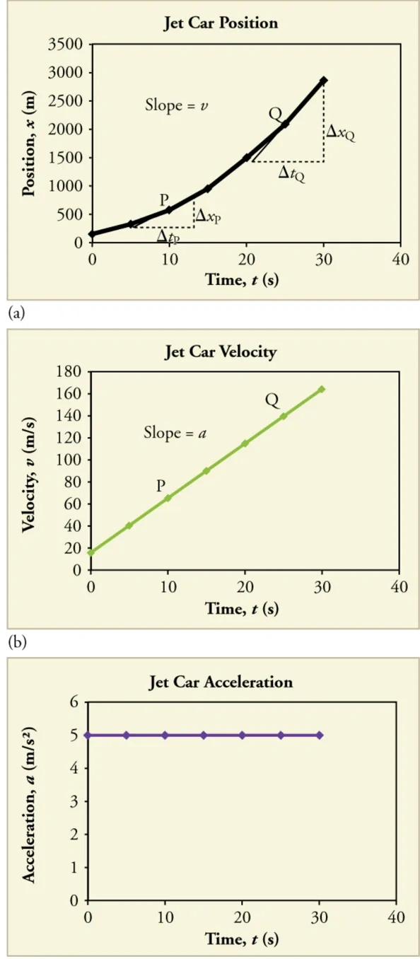
◀ Previous2 / 2
Photograph of a U.S. Air Force jet car speeding down a track, the kind of vehicle whose motion these graphs describe. Image: OpenStax, College Physics for AP Courses 2e, CC BY 4.0.
Instantaneous velocity from a curved position graph
 ⤢ Enlarge
1
When the car speeds up, its position-versus-time graph is a curve rather than a straight line. The slope of the curve becomes steeper as time passes
which shows that the velocity is increasing. The slope at any point on a position-versus-time graph is the instantaneous velocity at that point, meaning the velocity at that exact moment.
2
To find the instantaneous velocity, draw a straight line tangent to the curve at the point of interest
which means a line that touches the curve at that point only, and take the slope of this straight line.
3
If this is done at every point on the curve and the values are plotted against time, the result is a graph of velocity versus time.
4
The slope of that velocity graph is the acceleration.
Velocity versus time and acceleration
1
On a graph of velocity versus time, the rise is the change in velocity Δv and the run is the change in time Δt. The slope is therefore the acceleration, a = Δv / Δt, measured in m/s2.
2
Rule: The slope of a graph of velocity v versus time t is acceleration a.
3
Because the velocity-versus-time graph of the car is a straight line, its slope is the same at every point. This means the acceleration is constant, and the acceleration-versus-time graph is a horizontal line.
4
Using the straight-line form with velocity on the vertical axis, the intercept v0 (the initial velocity), the slope a and the horizontal axis t gives v = v0 + at. This relationship between velocity, acceleration and time has been obtained from a graph, and it matches the equation derived algebraically in the constant-acceleration section.
5
The same equations come out of graphical analysis as out of algebra. This is an important way physical relationships are discovered. Quantities are measured, one is graphed against another, and any correlation may suggest a relationship. Smooth graphs can then suggest a mathematical form
which further experiments test.
1Graphs of motion where acceleration is not constant2Graphs of motion where acceleration is not constant
Graphs of motion where acceleration is not constant
Graphs of motion where acceleration is not constant
Now consider the jet car as it goes from 165 m/s to its top velocity of 250 m/s.
Time again starts at zero, and the initial velocity of 165 m/s is the final velocity from the previous motion.
The acceleration starts at about 5 m/s2 and gradually decreases to zero when the car reaches 250 m/s.
The velocity keeps increasing until about 55 s and then becomes constant
because the acceleration is zero from 55 s onward.
1 / 2Next ▶
Velocity against time for the jet car levelling off at its top speed, and the matching acceleration against time falling to zero. Image: OpenStax, College Physics for AP Courses 2e, CC BY 4.0.
Graphs of motion where acceleration is not constant
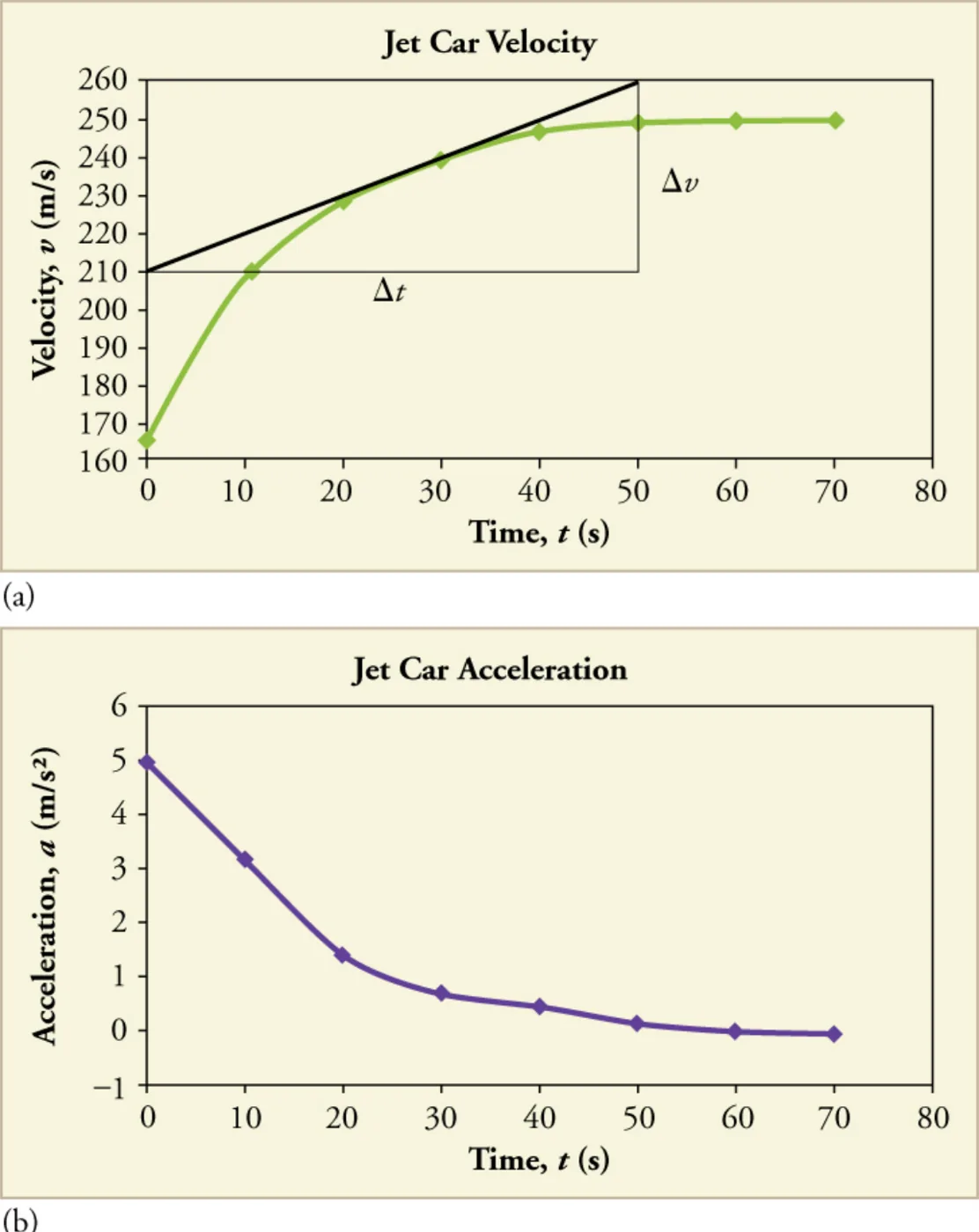 ⤢ Enlarge
Graphs of motion where acceleration is not constant
The slope of the velocity graph is the acceleration, and the acceleration graph is the result of finding that slope at every point. When the acceleration drops to zero, the velocity levels out. This makes the position-versus-time graph almost a straight line, with only a slight curvature that would be visible on a close-up.
◀ Previous2 / 2
Generating graphs from graphs
Generating graphs from graphs
A graph of position versus time can be used to generate a graph of velocity versus time, and a graph of velocity versus time can be used to generate a graph of acceleration versus time.
This is done by finding the slope of the graph at every point.
If a graph is linear, with a constant slope, the slope is easy to find and is the same for every point.
Graphical analysis can describe both specific and general features of kinematics. Graphs are also used in other areas of physics, and an important part of exploring physical relationships is to graph them and look for the underlying pattern.
1Check your understanding2Check your understanding
Velocity against time for a ship that moves at constant speed, then slows at two different rates until it stops. Image: OpenStax, College Physics for AP Courses 2e, CC BY 4.0.
Check your understanding
 ⤢ Enlarge
Check your understanding
A graph of velocity versus time for a ship coming into a harbor is shown below. (a) Describe the motion of the ship based on the graph. (b) What would a graph of the ship’s acceleration look like?
Answer (a): The ship moves at a constant velocity first
then begins to decelerate at a constant rate. At some point its deceleration becomes smaller, and it keeps this smaller deceleration until it stops moving.
Answer (b): The acceleration graph has zero acceleration during the first, flat part
where velocity is constant. It then shows a constant negative acceleration of larger size during the steep part, and a constant negative acceleration of smaller size during the shallow part, until the ship stops. The steps are sketched below.
1 / 2Next ▶
Acceleration against time for the ship: zero at first, then a larger negative step, then a smaller negative step. Image: OpenStax, College Physics for AP Courses 2e, CC BY 4.0.
Check your understanding

◀ Previous2 / 2
1Example 2.17: Determining average velocity from a graph of p2Example 2.18: Determining instantaneous velocity from the sl3Example 2.19: Calculating acceleration from a graph of veloc
Example 2.17: Determining average velocity from a graph of position versus time (jet car)
1
Problem: Find the average velocity of the car whose position is graphed in the first position-versus-time figure above.
2
Strategy: The slope of a graph of x versus t is the average velocity
because slope is rise over run, and here the rise is Δx and the run is Δt.
3
Because the slope is constant, any two points on the line give the same answer.
4
Widely separated points are the most accurate
because reading errors become proportionally smaller over a longer interval.
5
Solution: Choose the points (0.50 s, 525 m) and (6.40 s, 2000 m). Use final minus initial values: Δx = 2000 m − 525 m = 1475 m and Δt = 6.40 s − 0.50 s = 5.90 s. Then vavg = Δx / Δt = 1475 m / 5.90 s = 250 m/s.
6
Discussion: 250 m/s × 3.6 = 900 km/h, or about 560 mi/h. This is much greater than a typical highway speed limit of 60 mi/h (27 m/s, or 96 km/h)
but less than the record speed of 343 m/s (1234 km/h, or 766 mi/h) set in 1997.
1 / 3Next ▶
A curved position-against-time graph with a tangent line drawn at one point, whose slope gives the instantaneous velocity. Image: OpenStax, College Physics for AP Courses 2e, CC BY 4.0.
Example 2.18: Determining instantaneous velocity from the slope at a point (jet car)
 ⤢ Enlarge
Example 2.18: Determining instantaneous velocity from the slope at a point (jet car)
Problem: Calculate the velocity of the jet car at 25 s by finding the slope of its position-versus-time curve.
Strategy: The slope of a curve at a point equals the slope of a straight line tangent to the curve at that point. The point Q in the figure below is at t = 25 s.
Solution: The tangent line passes through two points, at 19 s with a position of 1300 m and at 32 s with a position of 3120 m. Δx = 3120 m − 1300 m = 1820 m and Δt = 32 s − 19 s = 13 s. Then v = Δx / Δt = 1820 m / 13 s = 140 m/s.
Discussion: This is the velocity given in the table for 25 s, and it is plotted on the velocity graph. The whole velocity-versus-time graph can be built in this way, point by point.
◀ Previous2 / 3Next ▶
Example 2.19: Calculating acceleration from a graph of velocity versus time (jet car)
1
Problem: Calculate the acceleration of the jet car at 25 s by finding the slope of its velocity-versus-time graph, shown in the figure of the top-speed motion above.
2
Strategy: The slope of the curve at 25 s equals the slope of the tangent line at that point.
3
Solution: The tangent line runs from (0 s, 210 m/s) to (50 s, 260 m/s). Δv = 260 m/s − 210 m/s = 50 m/s and Δt = 50 s − 0 s = 50 s. Then a = Δv / Δt = 50 m/s / 50 s = 1.0 m/s2.
4
Discussion: This value agrees with the acceleration plotted at 25 s on the acceleration graph
which is roughly 1 m/s2.
◀ Previous3 / 3
Key terms
| Term | Meaning |
|---|---|
| Straight-line graph | A graph in which the dependent variable changes by a fixed amount for each unit change in the independent variable, so the plotted points lie on one straight line. |
| Independent variable | The quantity plotted on the horizontal axis that is chosen or controlled, such as time. |
| Dependent variable | The quantity plotted on the vertical axis that responds to the independent variable, such as position. |
| Slope | The rise divided by the run of a straight line, which is the change in the vertical quantity divided by the change in the horizontal quantity. |
| Rise | The change in the vertical-axis quantity between two points on a line. |
| Run | The change in the horizontal-axis quantity between two points on a line. |
| y-intercept | The point where a line crosses the vertical axis, which is the value b in y = mx + b. |
| Average velocity | The change in position divided by the change in time, which is the slope of a position-versus-time graph over an interval. |
| Instantaneous velocity | The velocity at a single moment, which is the slope of the position-versus-time graph at that point. |
| Tangent line | A straight line that touches a curve at one point and has the same slope as the curve at that point. |
| Acceleration | The rate of change of velocity, which is the slope of a velocity-versus-time graph. |
| Constant acceleration | An acceleration that does not change over time, shown by a horizontal line on an acceleration-versus-time graph. |
1Avoid these mistakes2Avoid these mistakes3Avoid these mistakes
Avoid these mistakes
1Avoid this
Reading the slope of a position-versus-time graph as position. The slope gives velocity; the height of the line at a given time gives position.Avoid this
2Avoid this
Swapping rise and run, for example using Δt / Δx as the slope. Slope is always the vertical change divided by the horizontal change.Avoid this
3Avoid this
Using two distant points on a curve to get the instantaneous velocity. Instantaneous velocity needs the tangent line at the point of interest.Avoid this
1 / 3Next ▶
Avoid these mistakes
4Avoid this
Calculating a change as initial minus final. Always use final value minus initial value for Δx, Δt and Δv.Avoid this
5Avoid this
Thinking that zero velocity means zero acceleration.Avoid this
A ship can be at rest at the moment it stops and still have a nonzero slope on the velocity graph just before it stops.Avoid this
6Avoid this
◀ Previous2 / 3Next ▶
Avoid these mistakes
Forgetting the units shown on the axes, for example mixing km/h with m/s, or reading a time in minutes as seconds.Avoid this
◀ Previous3 / 3